


9. Electric and Magnetic Force Fields
10. Fields and Work
11. Potential
12. Electromotive Force
13. Faraday’s Law of Induction
14. Maxwell’s Equations and Electromagnetic Waves
15. Energy and Its Conservation
16.Force as a Potential Gradient
17. The Principle of Least Action
18. Lagrangian and Hamiltonian Mechanics
In the nineteenth century, investigations into electricity and magnetism led to the modeling of forces in terms of force fields
or fields,
whereby a distant source charge or current may qualitatively alter empty space. The field model would prove to be applicable to other kinds of force, including gravitation. Field theory has become a dominant mathematical paradigm in physics, to the point that most physicists speak of fields as if they were as physically real as the particles that are their sources. The question remains, however, whether the field is just a useful calculating tool or a real physical entity underlying seemingly non-local forces. To address this issue, we should look carefully at the physical basis for positing electric and magnetic force fields.
Electrostatics deals with the forces exerted by charged particles upon one another by virtue of their relative spatial positions. Electric charge is a fundamental property or quality of certain particles (e.g., electrons and protons) that is not reducible to any other property, as far as we know. Charge is a conserved
quantity, meaning that the total charge of any isolated system remains constant, which seems to imply that charge is real stuff
that cannot be arbitrarily created or destroyed. Even in exotic interactions where particles annihilate
each other, forming photons, the net charge is still conserved, since both annihilating particles were either neutral or of opposite charges, so the total charge is zero before and after collision. The fact that electric charge can be positive or negative, however, implies that this is not simply a spatially extensive measure of some corporeal quantity; it has a truly qualitative aspect. Yet perhaps the most fascinating thing of all about electric charge is that unlike mass, energy, velocity, and other basic kinematic properties, it is relativistically invariant, meaning that the observed charge of a system is the same in every frame of reference, inertial or otherwise. Not even Einsteinian relativity modifies the absolute measure of charge. If there is anything in physics that is really real,
charge would seem to be it.
Charged particles appear to exert forces on one another from a distance, following a law similar in form to that of gravitation. This law was discovered by Charles Augustin de Coulomb (1736-1806) in 1784. Coulomb’s Law, in modern notation, reads as F = kq1q2/r2, where q1 and q2 are the magnitudes of the charges (including their positive or negative sign), r is the radial distance between charges, and k is an arbitrary constant whose value depends on our choice of units. The strength of the force decreases with the square of the distance, as with gravity. When the charges are of opposite polarity (i.e., one is positive and the other is negative), the force is attractive, but when the charges are of the same polarity (i.e., both positive or both negative), the force is repulsive, which is never the case with gravity.
 Since both attractive and repulsive forces are possible in electrostatics, we can get much more complicated force interactions in multiple-body problems than we would with gravitation. Michael Faraday (1791-1867) introduced the use of
 lines of force
to depict the direction in which an applied force would act if a charged particle was there to be acted upon. In this way, one could map out all of empty space and see how hypothetical charged particles would be affected at different points in space. This convenient device has since been adopted by all physicists, who define the strength of an electric field
at each point in empty space to be the force applied on a hypothetical test charge of unit magnitude. Thus electric field strength is measured in units of force per unit charge (a common unit being the statvolt).
To this day, we have no empirical way of knowing whether an electric field is a physically real object or just a mathematical convenience. Those who hold an instrumentalist notion of science maintain that it does not matter, as long as the hypothesis of an electrical field works,
in the sense that it makes accurate quantitative predictions. Such an attitude essentially abandons philosophical realism in physics, and reduces physical theory to mathematical models that merely save the appearances.
Physically speaking, it makes a very big difference whether fields are real, since upon that hinges whether electrostatic forces are mediated by action at a distance or by direct local action. For his part, Faraday believed that his lines of force
corresponded to real entities that could affect the state of empty space.
 The supposition that a field is a physically real entity might help account for the inverse square of distance (1/r2) that we find in Coulomb’s law. The mathematician Karl Friedrich Gauss (1777-1855), using the assumption of a total constant flux of electric field from a charged particle, showed that the sum of the perpendicular force field integrated over any arbitrary closed surface surrounding the particle would be equal to the total charge times some constant. In other words, no matter how far away or how irregularly we draw our surface enclosing the particle, the total perpendicular force field, or flux, through that surface will remain constant. (The diagram shows some sample surfaces in cross-section. They completely enclose the source in three dimensions.) Note that Gauss assumed a constant total flux emanating from the source charge, so the proof of Gauss’s Law, like all mathematical proofs, is tautological in nature. Nonetheless, the subsequent empirical verification of Gauss’s Law shows that total flux does in fact remain constant at all distances. If electric field, with its associated flux, could be accepted as a real physical entity, we would have an intelligible explanation of the inverse-square force law. Since the area of a surface enclosing a source charge increases with the square of the distance, the flux density necessarily decreases with the square of the distance, since the same total flux must be spread out over an ever-increasing surface area. The inverse square law, then, is simply an artifact of geometry, combined with the assumption that some finite amount of electric flux
 emanates
from a source charge.
 A similar analysis can be applied to magnetism, which results from the effects of moving charges. There are two components to the force a moving charge exerts on another moving charge. First, there will be an electrostatic component, computed using Coulomb’s Law based on the positions of the charges at a given point in time. Second, there will be magnetic
 lines of force
or a magnetic field
generated by the motion of the first charge. However, unlike the case with electrostatics, these field lines do not point in the direction of the force experienced by the second charge. The direction of the force applied (F) is perpendicular to the plane formed by the already existing motion of the second charge (v) and the direction of the magnetic field (B). (In the diagram, charge Q2 is moving toward the reader, while Q1 applies an upward force F on Q2.) The magnitude of this force applied is equal to the charge times the magnetic field strength (i.e., the magnetic analogue of electrostatic force), times the component of the second charge’s velocity that is perpendicular to the magnetic field (F = q2v ⨯ B). The direction of force is reversed if the charge is negative.
The magnetic field B is a rather strangely defined field, since its direction does not match the direction of the force applied. Is this just an artifact of an odd choice of convention (defining the direction of the magnetic field as that in which no force is applied to a particle moving in that direction), or is there some reason to believe that something physically real, or at least as real as an electric field, points in the direction of B?
 A potent visual argument for the reality of magnetic fields is the fact that a bar magnet will align itself along the direction of a magnetic field line. We see this with the needle of a compass, and with iron filings on a piece of paper near a larger magnet (shown on left). The example of the compass is especially striking, since it responds even when it is remote from the magnetic poles of the earth. It would seem, then, that there is a field that acts immediately and locally on the magnet, unless we accept action at a distance. However, it must be remembered that magnetism is consequent to the internal electric flow within a substance, so we need not affirm that there is a magnetic field in addition to the constituent electric fields of the magnet and of the earth.
We can define a magnetic flux in analogy with the electric flux, yet our corresponding Gaussian law is only that the total magnetic flux through a closed surface is always zero. This is due to the fact that magnetic field lines never terminate at any source
or monopole, since magnetism, as far as we know, is only an artifact of moving electric charge, not the product of some other magnetic
kind of charge. This hardly assures us that the magnetic flux or magnetic field are physically real entities.
 There is, however, a law between magnetic field and current (rather than charge) that has some striking analogy with Gauss’s law. Electric current is itself a kind of flux, being the total amount of charge that passes through a given area per second. According to Ampère’s Law, the sum of the tangential component of the magnetic field along any closed curve surrounding a cross-section of the current flow generating that field will be constant, and proportionate to the magnitude of the current. Since charge is
 really real,
there is no difficulty in admitting that current, the movement of charge, is at least as real as any physical motion. The fact that the magnetic field encircling a current is always constant and proportionate to the current suggests that there might be something real pointing in the direction of the magnetic field as conventionally defined.
As with Gauss’s law, it is unclear whether Ampère’s Law deals directly with physical entities, or with mathematical abstractions only indirectly related to physical reality. André-Marie Ampère (1775-1836), unlike Gauss, was an experimentalist who confirmed his mathematical relation in the laboratory. Nonetheless, this did not prove that there really is such a thing as a magnetic field, only that it is a functionally useful model for describing physical reality. Such mathematical laws
were simply quantitative descriptions of how phenomena actually worked, but it was easy to elide into saying that the universal law is the reason or cause of particular phenomena exemplifying the relation.
We are nowhere near the exotic mathematical constructs of relativity and quantum mechanics, yet already it seems we may have drifted away from physically real agents to mathematical abstractions. If it was imprecise of Newton to ascribe causation to forces rather than bodies in motion, we are even further into the realm of abstraction when we deal with fields, which define how much force would be applied if something was there to receive it. We do not know if an electric field is a real physical entity, though the conservation of its flux might persuade us this is so. The physical reality of a magnetic field is even more doubtful, seeing that its direction does not even correspond to the force it supposedly engenders.
Still, most physicists, and even most laymen, act as if electric and magnetic fields are real physical entities. A sort of realism motivates this common sense understanding. When we repeatedly place an object in a certain location and it always moves the same way, we can hardly be blamed for supposing that that area of space has a special quality that causes this type of motion. The notion of a field, then, matches our physical intuitions about what we observe when we see magnets or static charges interacting. The two objects do not mystically leap at each other across the void, magically discerning where the other one lies, but rather one emanates a certain quality or power that alters space, subjecting objects there to an associated force.
This common sense
understanding of fields implies and arguably is informed by action by direct contact. The notion of a field allows particles to effectively act a distance, yet through a real physical agency that acts locally. If fields are physically real in the way described, it would seem to follow that they must emanate from their source in a continuous movement, for if the field were generated all at once, even in the furthest reaches of space, we would again have action at a distance. We will have to wait for twentieth-century physics and its notion of particle-mediated fields in order to explore the idea that fields are altered at a distance only after some finite time passes.
If fields can provide an intelligible physical model of apparent action at a distance for electricity and magnetism, it might do the same for gravitation. We could have a gravitational force field with force lines radiating from each massive object. In such a model, gravity alters the quality of empty space, so that the motion of massive objects is affected. Eventually, Einstein’s theory of general relativity would posit that gravity affects space in a far more fundamental way. Yet even with a classical field theory of gravity and electromagnetism, it should already be clear that there is no true void in space, which is in fact filled with fields.
How do these fields propagate across space? Most of space is certainly a void in the sense that it is occupied by no massive bodies, but might there not be some more aethereal substance that serves as a medium? This difficulty can help us appreciate that the nineteenth-century belief in a substantial electromagnetic medium or aether
was not an idle fancy, but was grounded in the belief that electric and magnetic fields are physically real entities occupying otherwise empty space. We will revisit the question of an electromagnetic medium later when we discuss Maxwell’s equations and electromagnetic waves.
If we accept the physical reality of fields, we can deduce an intelligible hierarchy of physical causes. We begin with electric charge as a brute fact or primitive quality of matter. By virtue of this quality, certain particles are able to act as sources of electric fields, which extend over large distances and exert force on other charged particles, altering their motion. Moving charged particles, in turn, generate magnetic forces and fields, which may alter the motion of other moving charged particles.
Interestingly, the forces associated with fields seem to be inexhaustible, as a field can repeatedly exert force on any charged particle that enters that region of space, without diminishing in intensity and without weakening the source charge. This is similar to gravitational force, which does not diminish in intensity nor cause the loss of mass. However, in a kinematic collision, the imparting of force causes the source particle to lose momentum. If all these different kinds of force have something in common, we need to make sense of these apparently contradictory accounts of their conservation.
The need for continuous application of force is by no means restricted to electric and magnetic fields. Fluid and air resistance can be modeled as the continuous application of force in a region of space, and the same may be said of surface friction as an object is dragged across the ground. To move an object in such conditions, it does not suffice to impart a one-time transfer of momentum to propel the object indefinitely. Rather, continuous application of force is required to overcome the resisting force, or motion will cease after some finite progress. This necessity is quite commonplace in terrestrial conditions, where all space is filled with gas or fluids or solids that resist moving objects. In fact, it is precisely for this reason that Aristotelian natural philosophers opposed Galileo’s inertial mechanics, which seemed to obtain infinite motion out of finite exertion, contrary to all terrestrial observation. The key to reconciling inertial mechanics with the observed limits of projectile motion, we have seen, is to recognize that force is proportionate to acceleration rather than velocity.
 We use the calculus of contour integration to give us the continuous sum of force applied over some path. In modern notation, this sum is written ∫CF⋅ds, where F is the force constantly applied, and s is the displacement along some path or contour C. We only count the force that is parallel to the direction of displacement at each point on the path. This sum of force applied across the distance traveled is known as mechanical work.
In the early nineteenth century, it became clear that the concept of work was a highly useful metric for the economy of physical interactions. Following our common-sense intuition that you can’t get something for nothing,
work measured how much motion one could get out of some finite application of force in a host of different circumstances. The mechanical work of a motor was measured by how high it could raise some weight, since such exertion required continuous opposition of the gravitational force. Later, James Joule (1818-1889) would demonstrate that mechanical work produced an equivalent amount of heat, suggesting that something more broadly energetic underlies the phenomenon of work. For now, we will look at how the concept of work can be applied to electric and magnetic force fields.
Since electric and magnetic fields involve a continuous application of force on a charged particle, we can use calculus to compute the work applied on any particle moving from point A to point B. Strikingly, we find that the work to get from A to B is the same regardless of the path chosen. This property of electric and magnetic fields, which is also shared by gravitational fields, will let us define what is known as potential.
When a field exerts the same amount of work upon an object to move it from point A to point B, regardless of path, we can know in advance how much work is needed to move the object to B, since the work is simply a function of the starting and ending positions. We could even map all of space in a given field, showing how much work is needed to go from any point to any other point. The way to achieve this is to define a quantity Φ called the potential at every point in space, where the difference Φ(A) - Φ(B) is the amount of work it would take to move an object from point A to point B. As force is applied continuously to an object, generating positive work, the object moves from a region of higher potential to one of lower potential. Indeed, the field’s applied force at any given point is equal to the negative gradient (rate of decrease per unit of space) of the potential.
A potential function can be defined not only for electric and magnetic fields, but for any conservative
force, that is, a force that applies the same amount of work to move from A to B regardless of path. One such force is gravitation, which we will use to give an illustrative example.
If an object of mass m is held some height h above the ground, the force of gravity (mg) will potentially be applied to it over the distance h it will fall, for a total potential work of mgh. Horizontal movement does not add any work, since there is no horizontal gravitational force (we ignore air resistance, since we are considering gravitation in isolation). Thus the gravitational potential at every point above the ground is mgh, where h is the height above the ground. Note that potential is defined relative to an arbitrary zero-point, in this case the ground.
With electric fields, we also define potential with respect to an arbitrary ground
or zero-point. However, following the convention of defining field strength in terms of force per unit charge, we measure electric potential as work per unit charge. As an absolute measurement, electric potential is completely arbitrary, due to the arbitrary choice of a ground or zero-point. However, as a relative measurement, it is as real as the work applied by the field to the test charge. In fact, we do not even need to insist that the field is physically real in order to acknowledge that real work is done to the charge, as long as we admit that force is physically real.
Electrical potential difference is what we ordinarily call voltage (after Alessandro Volta, inventor of the electric pile or battery), though a voltmeter does not measure potential directly. There are two basic ways to measure voltage. One is with an electrometer, which measures the relative quantity of charge at two different points (by measuring Coulombic displacement), from which we can calculate the potential difference. The more common method is to use a galvanometer (named after the 18th-cent. physicist Luigi Galvani), which measures the deflection of a moving coil interacting with a permanent magnet. The deflection is proportional to the current in the coil, which in turn is proportional to potential difference. Since the coil connects the two terminals of a circuit element, a current flows between them, lessening the potential difference. However, a resistor of high resistance can slow down this process, so that this effect is negligible, and we effectively measure the full potential difference to good approximation.
A voltage or potential difference of particular interest is that between the terminals of a battery or other power source. The two terminals have a potential difference due to excess positive charge on one terminal and excess negative charge on the other. In order to maintain this potential difference, a non-electrostatic force is needed to prevent the excess charge on each terminal from moving to the other terminal, via Coulombic attraction, which would make the whole battery electrically neutral, with no potential difference. This non-electrostatic force, which could be any mechanical, chemical or other force that prevents the terminals from discharging toward each other, must be equal and opposite to the Coulombic or electrostatic attraction, F = qE. This non-electrostatic force, being equal and opposite to a conservative force, is also conservative and therefore may be modeled as a field with a potential function. We need not assume that this field is physically real, but for our purposes need only point out that the amount of work needed to move a charge from point B to point A is independent of path. On an open circuit (where the terminals are not connected to each other by a wire or any other circuit elements), the work per unit charge applied by the non-electrostatic force must equal the work per unit charge, or potential difference, of the electrostatic force. The work per unit charge exerted by the non-electrostatic force is called an electromotive force.
The name electromotive force
is poorly chosen, since we are actually referring to the amount of work per unit charge, not force. Adding to the confusion, since the magnitude of the electromotive force (emf) is equal to the electrostatic potential difference between the two terminals, we can measure the emf in volts, and it becomes common to refer to the emf as simply the voltage or potential difference between terminals. Such usage makes it unclear that the emf is actually the work per unit charge applied by a force opposing the electrostatic force, and that the potential of the non-electrostatic force has a gradient in the opposite direction of the electrostatic potential. The potential difference or voltage that we actually measure across a battery is the electrostatic potential difference, not the emf. We happen to know, however, that the emf is always equal in magnitude to the electric potential difference, so in practice we often refer to the two equivalently.
The concept of electromotive force will help us understand Michael Faraday’s (1791-1867) findings regarding the interaction of magnetic fields and electric current. Significantly, he found that magnetic fields could induce electromotive force, an important discovery that would make possible the development of electric motors. The relationship between magnetic field and induced current may also give some insight into why the direction of the magnetic field does not match the direction of force applied to a moving charge.
 When a conductor is moved perpendicular to a magnetic field, the charged particles within it experience a force FB = qv ⨯ B, as described previously, in a direction mutually perpendicular to both the direction of motion and the direction of the field. If the direction of this force is along the length of the conductor, and we couple the ends of the conductor to the remainder of a closed circuit, the magnetically moved charge can create a current through the circuit. From this physical analysis we can see that magnetically induced current involves nothing other than the magnetic force described previously. Since this magnetic force moves the charge along a length of conductor l, the induced electromotive force, or work per unit charge, is FB⋅l/q = vBl.
As the conductor of length l moves with respect to the remainder of the circuit (see diagram), it makes the area of the circuit larger, thereby increasing the total magnetic flux through the circuit. Mathematical analysis of this variation yields Faraday’s Law of Induction, namely that the induced electromotive force vBl is equal to rate of change in magnetic flux. This is expressed in modern notation as: emf = dΦB/dt.
The fact that the induced electromotive force (work per unit charge) is equal to the change in magnetic flux suggests that magnetic fields are real physical agents, capable of performing work. After all, the amount of work done is proportionate to the total amount of magnetic flux enclosed by the circuit, suggesting that the entire field filling this space contributes to the work done. The phenomenon of induced current also supports our choice of convention for the direction of a magnetic field, since flux is necessarily perpendicular to the circuit loop in order to induce current. The deeper question of why magnetic fields exert force in an orthogonal direction remains a mystery, but this paradox is lessened if we accept that the magnetic field is a real causal entity distinct from the applied or induced force.
Magnetism, we recall, is itself produced by moving charge, and its direction is perpendicular to the motion of the charge and to the force it applies on other charges. In a sense, magnetism acts as a middle man
between a source current and an induced current. It is tempting to think that the intermediary of magnetism is just a mathematical formalism showing how moving charge can exert force in such a way that it moves other charges. However, the dependence of induced current on magnetic flux at least suggests, though it does not prove, that a spatially distributed magnetic field acts as a real physical agent.
Arguably stronger support of the notion that both electric and magnetic fields are physically real entities may be found in the way they interact directly with each other to form a propagating wave, observable as light and other kinds of electromagnetic radiation. A wave theory of light was made possible by James Clerk Maxwell (1831-1879), who supplemented Gauss’s Law, Ampère’s Law and Faraday’s Law with the insight that magnetic fields are similarly induced
by changes in electric field strength; and further that all magnetic fields are produced by electric currents. These insights yielded the famous Maxwell equations, which showed that even in a vacuum—i.e., a region where there is no moving charge—changes in electric field strength effectively constitute a displacement current
that can act as a magnetic field source. In this theoretical structure, Maxwell’s equations are not merely statements of quantitative equality, but relations between a source or cause and its effect. If the reader will excuse the intrusion of vector calculus notation (curl,
div
), we can see this below:
curl E = -(1/c)(dB/dt)
curl B = (1/c)(dE/dt) + 4πJ/c
div E = 4πρ
div B = 0
In each of these equations, the right side represents the source of the phenomenon represented on the left side. First, we have Faraday’s law, showing how change in magnetic flux induces an electric current in a circuit around the direction of the magnetic field. Second, we see that a magnetic field can be induced by the movement of charge, as was already known by Ampere’s Law, yet Maxwell showed it could also be induced by a change in electric field strength (dE/dt). Next we have Gauss’ famous relation between charge density and electric flux. Again, causality is from right to left, since the electric field is produced by the charge, not the charge by the electric field. Lastly, in the fourth equation shown, Maxwell postulated that there is no magnetic equivalent of a source charge or magnetic monopole.
This means that all magnetic fields are the product of electric fields or electric currents, a finding that proved to hold under experimental scrutiny, as it came to be understood that permanent magnets are magnetized
by virtue of moving charges at the molecular level and below.
A propagating wave in empty space, consisting of an electric field of sinusoidally varying intensity, and a magnetic field in the perpendicular plane (both fields being orthogonal to the direction of propagation) will satisfy Maxwell’s equations if the electric and magnetic fields are of equal intensity, and the speed of propagation is c, the speed of light. Thus electromagnetic radiation, including light, can be modeled as a perturbance in an electric field and an associated magnetic field. This would seem to suggest that fields really do alter space, which may be considered as a plenum, and that disturbances in empty space
(regions void of massive or charged particles) can propagate as real entities (for surely light is a real physical agent), suggesting that empty field-altered space acts as an aethereal medium. It is no wonder, then, that the theory of a plenum or aether experienced a resurgence in the nineteenth century.
We can now amplify the theory of causality for electromagnetism. Electric charge creates electric fields, but there is no such thing as magnetic charge.
Instead, magnetic fields are generated by moving electric charge or by changes in electric field strength (which necessarily result from some moving charge). Changes in magnetic field strength, in turn, can induce an electric field. Oscillatory disturbance in electric and magnetic fields can manifest themselves as energetic propagating waves. Their speed of propagation, the speed of light c, is a constant built into the relationship between the rate of change in field strength and the magnitude of the induced field.
Intriguingly, Maxwell’s equations deal only with fields, not with work, potential, or electromotive force, yet they give a mathematically exhaustive account of classical electrodynamics. This suggests that work, potential and emf (which is just work per unit charge) are not necessary causal agents. Indeed, this ought to be the case, since the work
is not that which does something, but a measure of that which has been done, and potential is just a measure of how much work will be done. Forces remain the only real causal agents, as in Newtonian mechanics, except now they are mediated by fields rather than direct corporeal contact. If we are to follow the greater philosophical precision of the Scholastics, we should say that forces are not causal agents, but acts of some agent. Our explorations of electromagnetism strongly suggest that not only corporeal particles may act as physical agents, but also electric and magnetic fields, as is most eminently the case in propagating waves of light.
Although work and potential are not needed to give a causal account of electromagnetism, they figure prominently in developing a theory of energy, whereby we can account for the economy of physical interactions. As noted previously, a continuous application of force in a field accomplishes a finite amount of work. Nineteenth-century discoveries in thermodynamics would make clear that mechanical work was convertible to other forms, including heat, suggesting that various physical processes were manifestations of a quantifiable energy,
defined broadly as a physical capacity to perform work. Significantly, energy proved to be a conserved quantity, suggesting that it was a substantial entity underlying all physical activity. Indeed, the Law of Conservation of Energy was a fundamental tenet of nineteenth-century physics, and it was frequently interpreted in a materialistic way, as if energy was some amount of stuff
that could not be created or destroyed. Many intellectuals pretended that the law had a broader philosophical application, invoking it as a scientific proof against the possibility of supernatural occurrences. Such metaphysical naivete will not suffice for our analysis, so we will scrutinize the empirical basis for the notion of energy more closely.
In Aristotelian philosophy, energeia was the actualization of being, or the realization of some potential, power or capacity, called dynamis. This distinction between the potential and the actual was crucial to Aristotle’s analysis of change or motion on a metaphysical level, as it resolved the false paradoxes of the pre-Socratic philosophers. The early modern mathematician and physicist Gottfried Leibniz (1646-1716), well versed in Scholastic concepts, applied the classical distinction between potentiality and actuality to the new mechanics. He identified the product mv as dead force
(vis mortua), while he called the quantity mv2 a living force
(vis viva). Neither of these quantities have dimensions of force. The first, which is momentum, is an inertial kinematic property of an object, so Leibniz called it dead.
The latter quantity has dimensions of work, so it represents kinematic force in action. It would become the basis of what we now call kinetic energy.
From Newtonian mechanics, we know that force equals the rate of change in momentum over time, or F=dp/dt. This enables us to express work as:
∫F dr = ∫(dp/dt)dr = ∫m(dv/dt)vdt = (m/2)∫(d/dt)v2dt = (m/2)(vf2 - vi2)
This means that the work done by a mechanical force equals one half times the mass times the difference between the final velocity squared and the initial velocity squared. The work done equals the increase in the quantity (1/2)mv2, where v is the velocity of an object at a given instant. We may call this quantity kinetic energy,
signifying how much work has been put into the motion of an object.
Unrealized or potential work is not momentum (mv), as Leibniz thought, but the potential function for whatever external force might be applied to an object. We have already discussed gravitational and electric potential. Now we will see how such potentials can be applied to objects in a way that increases their kinetic energy.
Using the simple example of a uniform local gravitational field, consider an object at height h above ground. The gravitational potential is mgh. Its velocity is zero, so its kinetic energy is zero. When it has fallen the entire height h, the potential has dropped to zero, while its velocity can be computed as follows.
The distance s that a constantly accelerating object travels as a function of time (t) may be expressed as:
s(t) = v0t + (1/2)at2
where v0 is the initial velocity and a is some constant acceleration. In our example, we take v0 to be zero, and the acceleration to be that of Earth’s gravitation near the surface, g. At the final instant tf, the distance traveled will be h, so we can write:
s(t) = h = (1/2)gtf2
From this, we can solve for tf algebraically:
tf = √ 2h/g
Now that we know the amount of time elapsed during the object’s fall, we can compute the final velocity vf:
v(tf) = gtf = g √ 2h/g = √ 2gh
From the final velocity, we can calculate the final kinetic energy Tf:
Tf = (1/2)mvf2 = (1/2)m(2gh)
= mgh
As the object falls, the potential decreases from mgh to zero, while the kinetic energy increases from zero to mgh. We might therefore see the act of falling as a conversion of the potential into kinetic energy. Note that it does not matter what we choose as the zero point for the potential, nor what we choose for the initial velocity of the falling object, since our result affects only the change in potential and the change in kinetic energy. Our result shows that a decrease in potential is matched by an increase in kinetic energy, so that, in a given reference frame, the total energy (kinetic plus potential) remains constant.
This conservation of total energy holds for any system where all forces can be expressed in terms of potentials. As noted previously, this is true for any force that exerts the same amount of work to move an object from point A to point B, regardless of path. Such a force is called a conservative force. We can generalize even further, and consider a system of many particles, with internal forces between these particles and external forces applied from outside the system. As long as all the external and internal forces are conservative, we will have conservation of total energy.
This thesis, which involves no mathematical formulae beyond what can be derived from Newtonian laws, has astoundingly broad implications, when we consider that all the fundamental forces of physics are conservative. Only on the macroscopic scale do we find non-conservative forces such as friction, yet even these convert potential into kinetic energy, except they do so on a microscopic scale and in a dissipative manner (e.g., as vibrating atoms or heat), rather than in a single direction. It would seem, then, the energy conservation is a universal law.
It is tempting to infer that the Law of Conservation of Energy implies that energy is the real stuff
of action, something that can neither be created nor destroyed, but only transferred from one operation to another. This was indeed the dominant interpretation of the nineteenth century, which seemed to receive further confirmation in James Joule’s discovery of the mechanical equivalent of heat. Mechanical energy dissipated into a liquid could raise the temperature of that liquid by a calculable amount, so that the total increase in heat corresponded to the mechanical energy put into the system. Indeed the study of thermodynamics would provide a fully generalized analysis of energy, which we will examine later.
Before we get carried too far, we should recall that neither potential nor kinetic energy are absolute quantities. Potential depends on the choice of an arbitrary zero-point, and kinetic energy depends on velocity, which is relative to one’s choice of reference frame. Thus total energy, which is just the sum of potential and kinetic energy, cannot have an objective absolute quantity. The Law of Conservation of Energy only tells us that there can be no increase or decrease in this quantity in a given frame of reference, for an isolated system. By isolated,
I mean that no particles or radiation (carriers of energy) are allowed to enter or leave the system. Yet even non-isolated systems are subject to the Law in a more general sense, since any physical entity added or subtracted will be subject to conservative forces, so the augmented system (including all remotely interacting entities) will have constant energy. As a corollary, the entire universe cannot increase or decrease its total energy. Nonetheless, this does not prove that energy is a physical substance or a primary quality of substance.
One component of energy, the potential, is derived from the notion of force fields qualitatively altering space. Even if we accept that a field is more than a convenient mathematical model, it does not follow that the potential is anything more than a convenient device for computing the work exerted by a field between any two points. Still, we might be persuaded of the physical reality of potential by the all-too-convenient physical fact that all fundamental forces are conservative, and thus have definable potentials. Yet it remains to be clarified: of what is potential a property, or is it a substance?
Potential, if it is physically real, would appear not to be a property of any determinate object, since its value is the same regardless of whether a hypothetical object to be acted upon is present or not. It would seem, then, to be a property of empty
space, or rather of the field that has altered that region of space. Being a purely relative quantity, it is difficult to conceive it as corresponding to some amount of substance, since there is no objective distinction among positive, negative and zero potential. Does potential generate the field or does the field generate potential? Recall that both fields and potential have fundamental particle properties (e.g., mass, charge) as their source. In the case of fields, we were able to give a plausible physical account by assuming that the flux is a real physical entity emanating from a source charge, though we cannot prove that this is the case. At any rate, this is better than we can do for potential, so potential, if it is physically real, probably ought to be conceived as derivative of a field, rather than the other way around.
What about purely kinematic potential? Does that really exist? Consider again the gravitational potential, mgh, which is supposedly converted into kinetic energy as an object falls. We might view this potential work as energy that is somehow latent in the gravitational force field. When an object is released from some height h, it acquires an increasing velocity, such that the total energy, E = (1/2)mv2 + mgh, remains constant. As the falling object accelerates, the kinetic energy increases and the potential energy decreases, yet the total remains constant, so we may see this as potential energy being converted into kinetic energy. This presumes that kinetic energy, (1/2)mv2, is a substantial entity. Such an assertion was uncontroversial in the nineteenth century, since both mass (m) and velocity (v) were assumed to be absolute quantities in Newtonian space and time.
Even if we do not yet consider how Einstein’s relativity makes mass and velocity purely relative quantities, it is still problematic to consider a field as storing some fixed quantity of energy. After all, the same field may act innumerable times on whatever particles happen to pass through it over the course of aeons, so that it does a practically limitless amount of work. What is finite is the amount of work required to move a particular object some finite distance. Potential measures this work before it actually happens, so it is aptly named, as it describes the potential of a field to perform work. To speak of potential as an existent physical entity would be to regard the potential as actual. Modern physicists often fail to recognize that existence is not the only mode of being, though quantum mechanics has helped lessen this naivete for some.
Another reason for doubting the physical existence of potential is that its magnitude can be arbitrarily defined, without any absolute zero-point. In the case of gravitational potential, h is defined with respect to wherever we expect something to break the object’s fall, e.g., the ground. It would be bizarre, then, to consider the potential mgh to represent a real amount of energy that is hovering in the gravitational field or in the falling object. This amount cannot be defined objectively, since the magnitude of the potential depends on where we locate the ground, even though the falling object is nowhere near the ground yet. Other kinds of potential are equally arbitrary, and in relativity the classical potential cannot even be defined at all.
Force is a change in momentum over time, or at any rate it is proportionate to the magnitude of momentum change. Energy or work is measured by integrating force continuously over an object's path. Interestingly, the form of the kinetic energy, (1/2) mv2, is equal to ∫mvdv or ∫pdp, that is to say, the integral of momentum over variations in velocity. Momentum, therefore, could be seen as a mathematical gradient or change in energy over velocity.
The concept of a gradient is useful for modeling the relationship between energy potentials and force fields. The force can be considered the negative gradient of the potential; that is, the strength and direction of the force matches the decrease in potential from one point in space to the next. If we can map the magnitude of the potential at every point in space, we can infer the strength and direction of the force field everywhere.
 Taking the simple example of gravitational potential, we can map the magnitude of potential at every point in space. Since the gravitational potential is mgh, where h is the height of an object above the ground, the potential in standard units equals 2mg two meters above the ground, 3mg three meters above the ground, and so on. At any given elevation, the potential remains constant in the horizontal direction, so there is no horizontal gradient, i.e., no horizontal force. In the vertical direction, there is a uniform gradient, as the potential decreases linearly with elevation, at a rate of mg per unit distance. Thus, the negative gradient or gravitational force is mg in the downward direction at every point. (On a large scale, we would have to consider that gravitational acceleration g varies with the distance from the earth's center.)
It is much more common to model forces as potential gradients in electrodynamics, where fields are practically indispensable. Yet here the potential does not, strictly speaking, have units of energy, since field strength is measured in terms of force per unit charge. Thus an electric potential has dimensions of energy per unit charge. In standard units, we measure potential as volts, and a volt is a joule per coulomb; that is, energy per unit of charge. When we speak of the voltage
across an element of an electrical circuit, we are actually speaking of the potential difference between two points. It does not matter that absolute potential has no objective reality, since it is only the relative difference in potential that suffices to account for the behavior of the circuit element.
Earlier, we posited charge as the physically real thing that causes electric and magnetic interactions. It may act on other charged particles either by applying force from a distance, or through the mediation of a real field that alters the quality of empty space (empty,
that is, with respect to mass). If the mathematical construct called potential
were taken as representing a real physical entity, the field strength might be considered nothing more than a gradient drop in potential. Such a model works fine for electric fields, but with magnetic fields, as noted previously, the direction of the force applied is not the same as the direction of the magnetic field. If the magnetic field strength is nothing more than a drop in some physically real magnetic potential,
it remains inexplicable that the direction of force should be different from the drop in potential.
Setting aside this difficulty, we can still compute a magnetic scalar potential
in analogy with the electrostatic potential. This magnetic scalar potential is a function with a defined numeric value at every point in space, such that the negative gradient of this function equals the magnetic field strength and direction. A magnetic scalar potential is definable for any magnetic field since magnetic force is conservative,
so that the same amount of work is applied to move an object from point A to point B regardless of path. Although the magnetic field direction is different from that of the magnetic force applied, this difference is always 90 degrees in the same relative direction, and the magnitude of the field is always proportional to the magnitude of the magnetic force. This has the mathematical consequence that the magnetic field retains the properties of a conservative vector field whenever the magnetic force is conservative, so that a scalar potential is definable.
I should like to address a bit of nonsense that is often proffered even by knowledgeable physics students, namely the notion that magnetic fields do no work,
and so are always conservative, since the work done around a closed loop is always zero. This bit of sophistry is a consequence of the fact that the magnetic field is formally defined to be perpendicular to the direction of the magnetic force, so indeed there is no work done in the direction of the magnetic field. However, as indicated above, the magnetic field and magnetic force are mathematically linked in a way that each can be represented as a conservative vector field if and only if the other is conservative. Further, the only reason a physicist should care about magnetic fields is because he believes them to be mathematically or physically linked to magnetic forces. Since magnetic forces certainly exert work, any attempt to disconnect magnetic fields from work done would necessarily entail disconnecting magnetic fields from magnetic forces, in which case magnetic fields are physically useless.
That being said, we should note that magnetic fields and forces are not conservative in general. This is because the presence of moving charge (i.e., electric current) can alter magnetic effects so that the curl of the vector field is non-zero. This has the mathematical consequence that the vector field cannot be represented as the gradient of a well-defined scalar potential function. Now, since there is, as far as we know, no such thing as a magnetic monopole (i.e., magnetic charge
), the only possible source of a magnetic field or force is electric current. This means that in actuality we can never expect magnetic forces to be conservative, though they may seem conservative to good approximation at some distance from the source current.
Since magnetic fields are generated by a moving source charge or current, it is useful to define a vector potential
in addition to the ordinary scalar potential. This vector potential has both magnitude and direction at every point in space, unlike scalar potentials, which are simply numeric. The vector potential A is defined by the formula B = curl A, where B is the magnitude and direction of the magnetic field. B is always the curl of some other vector field A as a mathematical consequence of the fact that the divergence of B is zero everywhere. The formula div B = 0, we may recall, is the expression of Maxwell’s postulate that there are no magnetic monopoles in nature. (The div
of a vector field measures how much the field lines diverge or converge at a given point in space.)
The curl
of a vector field, roughly speaking, is the amount of rotation in three dimensions the field would impart on a body if it represented a force. The components of the curl are calculated by taking the slopes with respect to pairs of cyclically permuted dimensions. (For example, the slope in the third Cartesian dimension with respect to the second minus the slope in the second dimension with respect to the third gives you the component of the curl in the first dimension.) Accordingly, curl is only definable in three dimensions, not two or four or any other number. This means magnetic vector potential is only definable in three dimensions. (Readers may recall that two of Maxwell’s equations, dealing with the induction of electric field by magnetic field changes and vice versa, also involved curl and therefore are definable only in exactly three dimensions.)
There are many different possible vector fields that could satisfy the right side of the equation B = curl A for a given magnetic field B. There will always be at least one such vector field A that has a divergence of zero. Even then, an A that satisfies both B = curl A and div A = 0 is not unique, because you could always add to A some other vector field A' with a curl of zero, and that would also be a solution. Vector potentials are used as mathematical conveniences to solve certain kinds of electromagnetic problems, and it is far from obvious that we should consider them to be real physical entities. However, the use of vector potentials leads to an important insight.
Recall that the electric, gravitational, and other scalar potentials have no well-defined zero point, meaning we can add any fixed number to the potential and still get the same result for the gradient or force field. This is why we can choose any arbitrary definition of what is ground
or zero potential
in electrostatic problems and still get the same correct results. With magnetic vector potential, instead of some fixed number, we can add any vector field with curl zero to the potential, and still compute the same result for magnetic field strength. It can be mathematically proven that any vector field which is a gradient of another vector field will have curl zero. So for any arbitrary vector field Λ (Greek letter lambda), it will always be true that A and A + grad Λ can both serve equally well as potential functions for the same magnetic field B.
If we decide to switch from A to A + grad Λ, this is known as a gauge transformation. The fact that the field B remains the same under such a transformation is known as gauge invariance. The conditions under which fields are gauge invariant reveals mathematical symmetries in the structure of these fields. Gauge theory would not be popularized in physics until the 1940s, when it would come to be applied in quantum mechanics. Before we can get there, however, we will have to understand the broader notions of symmetry and invariance as they developed in the late nineteenth century. First, we will need some background leading up to these discoveries.
In the eighteenth and nineteenth centuries, parallel to the discoveries mentioned about electricity, magnetism, and energy, there were important mathematical developments in and outside of physics that would eventually reshape thinking about where the laws of physics came from. By around 1900, theoretical physics would become fully mathematicized, as mathematics would become a sort of metaphysics and mathematical structures were conceived as the deepest realities behind physical phenomena. It is no accident that this philosophical development paralleled the decline of systematic metaphysics in the nineteenth century, as well as the ill-fated attempt to mathematicize logic, which I critique in another work. Yet the idea that mathematical equations could substitute as metaphysical and physical causes was no invention of nineteenth-century secularists. It finds its roots in the Age of Reason, when it was still socially acceptable to offer theological explanations of the natural order. One important example of the elevation of mathematics to nearly divine status can be found in the principle of least action.
The principle of least action is grounded in the ancient Greek dictum, famously mentioned by Aristotle, that nature does nothing in vain and nothing superfluous. This belief that nature is economical was likely grounded in observations of plants and animals, which exhibit astounding resourcefulness and always act for a useful purpose. In the Christian era, including the Age of Reason, it was clearly understood that this economy was the result of Divine Intelligence. The metaphysical principle of natural economy was used by the mathematician Pierre de Fermat (d. 1665) to explain the law of refraction, declaring that light always follows the path that takes the least time. This least-time principle was praised by Leibniz, who saw in it confirmation of final causes in physics, since the light must know
in advance the best path.
A century later, Pierre Louis de Maupertuis (1698-1759) modified Fermat’s principle, while still upholding the underlying tenet that Nature always acts in the simplest possible manner to produce its effects.
He proposed in 1744 that light follows the path of least action, where action is proportional to the continuous product of distance and speed, which is ∫v ds in modern calculus notation. Maupertuis mathematically demonstrated that reflection and refraction could be explained by the principle of the least action, while Fermat’s least time principle was but a special case where the speed of light is constant. Maupertuis accordingly believed that his principle was more fundamental, and that the least time principle was but a particular consequence of the least action principle.
Note that Maupertuis uncritically assumed that the order of formal mathematical derivation necessarily reflects the order of metaphysical priority. This would remain a common method of interpreting mathematical physics throughout the modern era. Even today, physicists often assume that Equation B is derivable from Equation A
implies that The physical reality described by Equation B is caused by the physical reality described by Equation A,
though this does not logically follow.
Maupertuis recognized that his least action principle, like Fermat’s least time principle, still invoked final causes, since the light must know
in advance which path will make it use the least action. Nonetheless, he argued that final causes as such were not problematic; rather, we must not be too rash to identify a particular final cause as fundamental, when it is actually consequent to something deeper. Since the teleology inherent in Maupertuis’ least action principle was strongly deterministic, it amounted to a kind of fatalism. He suggested that there are two parallel aspects to the natural order, as governed by the Supreme Being. We could determine all the effects from a given state by studying the properties of material bodies and their forces, which manifest divine power. Alternatively, we could determine all effects equally well by considering what actions are most suitable for an object at a given point of time, which manifests divine wisdom. The least action principle was not intended to abolish the causal efficacy of forces in classical mechanics, but rather to complement this explanation of nature’s power with an explanation of its inherent economy or wisdom.
In the same year (1744) as Maupertuis, Leonhard Euler (1707-1783) independently arrived at a least action principle which was applicable to massive particles rather than light, and held only when energy was conserved. Euler’s action was similar to Maupertuis’, except it had a mass factor, so instead of ∫v ds, we have ∫mv ds, which is the integral sum of momentum (mv) over displacement (s).
The least action principle would obtain a more general form in classical mechanics after the Italian-born mathematician Joseph-Louis Lagrange (1736-1813) developed a powerful mathematical formalism for analyzing mechanical systems. Lagrangian mechanics minimized the number of variables one had to deal with, and eliminated explicit forces of constraint. This was useful in systems where mechanical variables are interdependent due to specified constraints.
To take a simple example, if two spherical objects A and B are connected by a rod, this constrains the position and velocity of one object with respect to the other. If we know the position of one object, we know the other has to be at some distance L, which is the length of the rod. Similarly, the velocities of the two objects are correlated. If we do not allow the rod to rotate (a further constraint), the velocities of the two objects must be equal. It is clear that with such a constrained system we do not need twelve different variables (the position and velocity of each object with respect to three coordinates) to determine the equations of motion. For example, if the velocities of the two objects are equal at all times, then we can eliminate the three variables of object B’s velocity, since those are equal to A’s velocity. Sometimes, however, it does not suffice to simply eliminate one of the variables in Cartesian coordinates. We may need to change coordinate systems in order to eliminate a variable. In our rigid body example, if the rod is allowed to rotate, we can eliminate a position variable is if we switch to a cylindrical or spherical coordinate system where the radial distance r from the center of the rod is one of the coordinates. For both objects A and B, that distance is always L/2, and never varies, so r can be eliminated as a variable, for both A and B. In fact, we can also eliminate the angle θ in a given plane for one of the objects, since, once we know the angle of one object, we know the angle of the other differs by exactly 180 degrees. Ideally, we want the only variables remaining to be fully independent of each other, in which case the number of variables is the number of degrees of freedom,
or dimensions in which change is permitted by the constraints.
Before Lagrangian mechanics, the standard way to solve problems involving constraints was to compute the forces exerted by the constraints and apply Newton’s laws. This could be extremely problematic in cases where the force varies with time. To take a relatively simple example, consider a bead that slides along a curved wire in a horizontal plane. Once we set the bead in motion with some velocity, it would tend to travel in a straight line, but the wire exerts a force that causes it to deviate from its straight-line path. This force of constraint changes over time, as the wire pulls the bead in different directions, and as the bead's preferred straight-line path changes with its own constantly changing direction of motion. If we could instead choose a coordinate system that measures position in terms of the distance traveled along the wire, we would have a much simpler mechanics problem, and could dispense with any time-varying forces of constraint. Since the wire could be curved any way we please, the coordinate system is also completely arbitrary.
Lagrange’s mechanical formalism uses generalized coordinates, typically denoted q1, q2, etc., which correspond to spatial displacement in some arbitrary direction that is specified according the computational needs of the problem. These generalized coordinates need not correspond to any of the mutually perpendicular x, y, z coordinates of Cartesian geometry, or those of any other conventional coordinate system. Lagrangian mechanics is widely used to this day by physicists to solve mechanical problems, and while it is a very powerful calculating tool, it can mislead us into confusing physical entities with mathematical contrivances.
Lagrangian mechanics is grounded in what is called d’Alembert’s principle, which in turn is derived from the principle of virtual work. Virtual work is mathematically similar in form to actual work, (described earlier), except it considers virtual displacement rather than actual displacement. This virtual displacement, denoted δr, is usually defined in physics textbooks as an arbitrary infinitesimal change of a system that occurs in zero time, which of course is absurd, since time must elapse for there to be change. A sounder explanation of virtual displacement has only recently been advanced by two Indian physicists (Subhankar Ray and J. Shamanna, Virtual Displacement in Lagrangian Dynamics,
1 Sept 2003). The virtual displacement may be defined as the difference between any two displacements of an object that are allowable under the constraints. For example, if a ball is constrained to roll along a surface, at a given point in time it may move in any direction on that surface. The difference between any two such displacements will necessarily be tangential to that surface. The force of constraint confining the ball to the surface is necessarily perpendicular to the surface, so the so-called virtual work
F δr must be zero, since no component of the force of constraint is parallel to the surface, while every virtual displacement δr is parallel to the surface.
The virtual work, so defined, is really a measure of how much work would be applied by a force if an object were to go in one allowable direction rather than another. Since the force of constraint indiscriminately allows movement in all directions on the surface, it would not exert any more or less work if the ball moved in one direction rather than another. Only in special kinds of constraints, like sliding friction, does the force of constraint involve non-zero virtual work. This is because the magnitude of the sliding friction force, though it is tangential to the plane of motion, is dependent on the magnitude of the normal (perpendicular) force, so a force of constraint effectively acts as an applied force doing work. We will ignore these kinds of constraints, and restrict ourselves to those where the net virtual work is zero.
A mechanical system is said to be in static equilibrium when the sum of all forces on each object in the system at a given instant is zero. It logically follows that the total net virtual work on each particle in such a system is also zero, since virtual work equals the product F δr. If we are dealing with a system where the forces of constraint have no net virtual work, then it follows that the net virtual work of any applied forces must also add up to zero, since:
(A) Virtual work of all forces = (B) Virtual work of applied forces + (C) Virtual work of constraint forces
We have just assumed that A and C are zero, so B must also be zero. The condition that B equals zero, or that there is no net virtual work by applied forces, is called the principle of virtual work.
We can use the principle of virtual work to devise a new form for the equations of motion that eliminates forces of constraint. In Newton's formulation, the equations of motion are given as F = dp/dt, or force equals the rate of change in momentum (p) with respect to time. We can rewrite this as F - dp/dt = 0. We may consider the term -dp/dt as a kind of force, at least for computational purposes, that opposes the actual force F. The sum of the actual force and this effective opposing force equals zero, so we may mathematically treat the system as if it were a mechanical system in equilibrium (all forces add to zero). The total virtual work (A) will be zero, and if we confine ourselves to systems where the constraints have no net virtual work (C), then it follows that the virtual work of the applied forces (B) will also be zero. The principle of virtual work for this system is: (F - dp/dt) δr = 0. This is known as d’Alembert’s principle, though it was Lagrange who first wrote it in this form. It differs from the principle of virtual work because here we are explicitly considering a dynamic (i.e., time-dependent) system. The mathematics from which it is derived is sound, but we should not think that the dp/dt term corresponds to a real force.
Starting from d’Alembert’s principle, Lagrange was able to derive equations of motion in terms of generalized forces in generalized coordinates. These generalized forces, denoted as Q rather than F, need not have dimensions of force, just as generalized coordinates need not have dimensions of linear displacement. The generalized forces
do not represent physical forces, but are mathematical contrivances that help us solve mechanical problems. In particular, Lagrange showed that, when the constraints are holonomic (dependent on position, but not velocity), the forces of constraint disappear, and we are left only with as many equations as there are independent variables, or degrees of freedom.
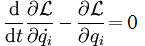
Lagrange’s equations of motion for systems with holonomic constraints are of the form:
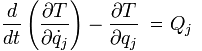
In these equations, the kinetic energy T is related to the generalized forces Q and generalized coordinates q. The kinetic energy T, unlike the generalized forces and coordinates, is not some arbitrary mathematical construct, but is in fact the classical physical kinetic energy, (1/2)mv2.
When the physical forces F can be expressed as the gradient of some scalar potential V (i.e., if the forces are conservative, as discussed previously), then the generalized forces can be expressed as the change in potential with respect to the generalized coordinates. Lagrange’s equations of motion can then be rewritten in terms of the function L = T - V, eliminating the Q. We do not care about Q anyway since it is not a real physical force.
The equations of motion in this form express the fascinating fact that the mechanics of a system with holonomic constraints can be fully analyzed in terms of generalized coordinates if we know the function L = T - V, called the Lagrangian.
What about forces that cannot be expressed as the gradient of a scalar potential? If the force could be derived from a generalized potential, denoted U, so that the force equals the negative gradient of U plus the time derivative of U’s gradient with respect to velocity, we could still have equations of motion in terms of the Lagrangian, except here the Lagrangian equals T - U. Here we are postulating a velocity-dependent potential, as opposed to the classical potential V which depends on position only. There is in fact a force of nature that can be modeled by a velocity-dependent scalar potential, namely magnetism.
For magnetism, a generalized potential U of the form just described will equal qφ - (q/c)A ⋅ v, where φ is the electric scalar potential, and A is the magnetic vector potential, discussed earlier. Note that U is not a physical potential (assuming that any potentials are physical), but is a useful construct that allows us to keep the equations of motion in a Lagrangian form.
Lagrange derived his equations of motion by considering virtual displacements as expressed in d’Alembert’s principle. In 1833, the Irish mathematician and physicist William Rowan Hamilton (1805-1865) showed that Lagrange’s equations could be derived from a different principle. If we assume that all applied forces can be modeled by generalized potentials like U (functions of position, velocity, and time), then the motion of the system from time t1 to t2 is such that the continuous sum of the Lagrangian over that time interval, ∫L dt, has a stationary value
for the correct path of the system’s motion. By stationary value,
we mean that if we were compare this value of ∫L dt to that for closely similar paths of motion, that we would be at a point where the rate of change in such values, comparing the actual path to closely similar paths, is zero. If we graphed a curve depicting the different values ∫L dt, the true path would be at a point where the slope of the curve was zero, namely at a maximum, minimum or inflection point.
This principle, now known as Hamilton’s principle, has some striking similarity to Maupertuis’ least action principle. Somehow the system knows
to prefer a path over some time interval that makes the slope of ∫L dt vanish, just as under Maupertuis’ principle an object takes the path that will minimize the action. In both cases, we are left with the perplexing problem of how the system could know
in advance which path will optimize a particular value over the long run. We should clarify that, in the case of Hamilton’s principle, optimizing ∫L dt need not mean minimizing its value, but only its slope, so it is not really a least action principle, but rather a stationary action principle. Still, the difficulty of apparent fatalism remains.
Some physicists today suggest that the least action principle should be the basis of Newtonian mechanics, since Newton’s second law can be derived from it, even though the least action principle does not deal with non-conservative forces. No matter, we are told, since the only non-conservative forces are not physically fundamental. Still, advocates of this view can give no reason beyond mathematical elegance for believing that this least or stationary action principle should be regarded as physically or metaphysically prior to Newton’s laws of motion.
Hamilton’s principle can be used to derive Lagrange’s equations, and vice versa, so it is not immediately apparent which of these should be regarded as more fundamental. At any rate, Hamilton proceeded to derive his own formulation of classical mechanics using his principle as a starting point.
In Hamiltonian mechanics, there are twice as many equations of motion as in Lagrangian mechanics, but they are simpler. The Hamiltonian equations of motion use a generalized momentum in place of the generalized velocities found in Lagrange’s equations. This canonical momentum
or conjugate momentum
is defined as the partial derivative (rate of change while holding variables in other coordinates constant) of the Lagrangian with respect to velocity along a given coordinate. If the coordinates are non-Cartesian, or if the potential is velocity-dependent, the canonical momentum
of Hamiltonian mechanics need not correspond to familiar Newtonian linear momentum. Hamilton’s formalism allows us to derive the equations of motion from the function known as the Hamiltonian:
H = T + V, the kinetic energy plus potential, or total energy of the system. Although solving problems with Hamiltonian mechanics is generally more difficult than using Lagrangian mechanics, it has the advantage of being theoretically more intuitive, since it makes the equations of motion derivable from the total energy of the system rather than the strange quantity T - V, and this function H is dependent on position and momentum rather than position and velocity with respect to generalized coordinates. The use of momentum is again intuitive, since that can be construed as the measure of how much motion
there is in Newtonian mechanics.
The use of Lagrangian and Hamiltonian formalisms to explain physical theory is fraught with dangers, however. We must recall that these are calculating tools filled with mathematical devices that do not necessarily correspond to physical entities. When we depart from Cartesian coordinates, the canonical momenta
of Hamiltonian mechanics need not have dimensions of physical momentum at all. Both Lagrangian and Hamiltonian mechanics may make use of a velocity-dependent generalized
potential U that is not a physical potential (if indeed there is such a thing). The fact that these mathematical formalisms work
is no proof that they are models of physical reality, only that they are effective calculating techniques.
The full significance of Hamiltonian mechanics would be expounded in the twentieth century, as it became clear that the Hamiltonian was useful for modeling quantum mechanical interactions, thereby serving as a sort of theoretical bridge between classical and quantum mechanics. Even from a purely classical perspective, Hamiltonian mechanics brings out important features of mechanical systems, as it can show certain symmetries. For example, if the Lagrangian is independent of a particular coordinate q, then the canonical momentum with respect to that coordinate is constant, or conserved. This correlation between geometric symmetries and conservation laws would be further explored in late nineteenth century and early twentieth century mathematics, leading to a re-evaluation of the significance of such laws.
Recalling that the canonical momentum, generalized coordinates and generalized potential are not necessarily physical quantities, we are struck by the fact that conservation laws with physical significance can be derived from relations among abstract contrivances. Realizations such as this have tempted physicists in the last century and a half to turn to a sort of Platonism or Pythagoreanism where we regard the mathematical or geometrical objects as more fundamental, while the physical laws are but consequences or expressions of this deep geometry. We will consider some of these developments more explicitly in the next chapter, as they would lead to the formal understanding of relativity and quantum mechanics that is accepted by most physicists to this day.
© 2010 Daniel J. Castellano. All rights reserved. http://www.arcaneknowledge.org
| Home | Top |