


For the less mathematically inclined, we provide a discussion of some statistical concepts. Readers more advanced in this area may wish to proceed directly to the next chapter.
Statistics deals with properties of collections of objects considered in aggregate. We take the measured values of some physical property (or more abstractly, a variable) for numerous individuals, and then make quantitative statements about the distribution of these values. It is often convenient to refer to each group of individuals with a universal term representing a class or set of objects. The use of universal terms does not mean that statistical statements should be interpreted categorically. For example, consider the true statement: Watermelons are larger than canteloupes.
This does not mean that any watermelon is larger than any canteloupe. Despite its syntactic form, we do not intend a categorical statement, but rather a statistical statement, i.e., that, on average, watermelons are larger than canteloupes.
That watermelons are bigger than canteloupes is a statement of statistical fact, not a normative judgment about desirability, nor a modal judgment about future possibilities. It is conceivable that we might breed watermelons to be smaller or canteloupes to be bigger, if for some reason we thought this inequality was a problem that needed to be solved. Yet breeding bigger canteloupes could be detrimental to their flavor, while breeding smaller watermelons might add to the cost of cultivation without much advantage in quality. It is not obvious that equality is always desirable or beneficial in nature.
Generally, inequality among individuals and groups is a biological necessity. It is such variation that gives evolution its matter to act upon. If there were no natural inequality, there would be nothing for natural selection to select. Selection is not an all-or-nothing process; many variations survive to greater or lesser degrees. Some disadvantage might be worth keeping for the sake of some concomitant advantage,[5] so a plurality of traits and property values may be retained in a population.
Statistical statements refer to properties of groups, not determinate individuals within those groups. Knowing all the statistical measures of a group need not tell you anything about a particular individual in that group or class. On the other hand, there could be no statistics without individuals, which are the primary existents. While it is common for scientists to disparage anecdotal
evidence as unreliable, this inverts sound ontology. In fact, scientific evidence is constructed from the aggregation of numerous cases, which individually prove nothing, but combine to give strong probabilistic evidence of a universal rule.[6]
Two statistical measures especially concern us: mean and variance. The mean (μ) is the arithmetic average value of some variable quantity across all individuals; i.e., the sum of these individual measures divided by the total number of individuals. For example, the mean of the data shown in the table below is 56, which is the sum of all values (1,120) divided by the number of data points (20). The variance (σ2) is the average of the squared difference between the mean and the measured value for each individual. Squaring ensures that this variance is always non-negative. The variance tells us how spread out
the values are from the mean. In the example, we take the difference between each value and the mean (56), and square it. Then we take the average of these figures for all points, which comes to 648.8. The square root of the variance is called a standard deviation (σ), another measure of the spread from the mean. Note that the standard deviation (25.47 in the example), when non-zero, is greater than the average distance of data points from the mean (21.7 in the example).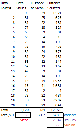
When a small subset of individuals varies greatly from the mean on one side but not another, this skews the distribution so that the average or mean value is not a good measure of the middle of the pack.
In such situations, it is preferable to use the median, which is the value greater than or equal to that held by half of the data points. When there is an even number of values, as in the example, we take the average of the two middle values (65 and 68). A common use of the median is in measuring income, since a few billionaires can skew the average upward, but the poor cannot have an income less than zero. The median gives a more typical
income for this group.
Sometimes a modest difference in mean (or median) between two populations can reflect a much larger difference at the extremes. For example, the average height of adult human males in the U.S. is 5′9″, while for females it is 5′4″. If you know nothing about someone besides their height, you cannot absolutely predict their sex. If the height is near the middle of the pack, like 5′6″, there is practically no predictive value of sex. If it is toward the upper extreme, such as 6′5″, the probability that it is a male increases. We note that differences are generally most pronounced at the extremes. In the U.S., 0.4% of men are over 6′5″, while only 1 in 800,000 women are above that height, which means there are about 3200 times as many men as women in that range. The truly exceptional cases may arise from random factors that do not correlate as neatly with sex. Only 95% of all people in the world who measured 7′6″+ were male, and the same is true for those were 8′+ in height (19 men to 1 woman).[7] The tallest man ever, Robert Wadlow, was 8′11″ tall, while the tallest woman ever, Zeng Jinlian, was 8′1¾″, yet she was only a couple inches shorter than Wadlow at the same age of seventeen. Nonetheless, for height ranges with significant sample sizes, the disparity tends to increase the further you get from the mean.
When the group of interest is the set of individuals measured, we do not have to wonder what the true mean and variance are. They are simply what we have computed. The only error or uncertainty in this value is from the measurement error in each data point. Assuming for simplicity that measurement error is the same value δ for all data points, then the error in the arithmetic mean is δ/√N, where N is the number of objects measured.
In most physical investigations, however, it is only practical to measure a tiny subset of the group of interest. This subset or sample is supposed to be representative of the broader group or population we wish to understand. It is important to select the members of this sample randomly, i.e., without regard for the particular value of the variable to be measured, or anything likely to be correlated to that value. When studying humans, we want a mix of races, sexes, and age groups, and preferably large numbers in each group, to make sure that oversampling from a particular group does not skew our result. For physiological measures, we are less likely to be concerned about irrelvant factors, such as whether the study is conducted in Pennsylvania or New Jersey. This is especially the case when dealing with more elementary physics, as we assume that electrons in one part of the world behave much the same way as in another part. This assumption of the uniformity of nature cannot be proven, but to date it has not been contradicted.
As we take larger and larger samples, they are more likely to have means that are ever closer to a limiting value, which we presume to be the true mean that we would compute if we could measure every possible member of a class or population. This central limit theorem applies only to normally distributed properties, i.e., those that have a bell-shaped distribution described by the Gaussian function:
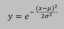
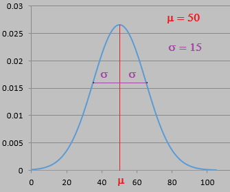
where μ is the mean and σ is the standard deviation. Fortunately, a normal distribution applies to most natural phenomena where the mean is much greater than zero (or else a Poisson distribution would be more appropriate) and there are no hard upper limits. If the distribution is skewed, the mean is not an appropriate statistic for characterizing the population; it might be better to use the median.
If we do not know the true mean a priori, we can nonetheless determine probabilistically, on the assumption that the population is normally distributed, that the sample mean (i.e., the arithmetic mean of values in the sample) is within some distance of the true mean. (There are other methods for different distributions, which need not concern us.)
If our sample is selected randomly, i.e., without regard for the values of the data points, then the sample mean μs is an unbiased estimator of the true mean μ, meaning that the probability-weighted average value of sample means equals the true mean. That is to say, if we could take the mean of every possible sample and then take the average value of these means (weighting the average if some samples are more probable), this would equal the true mean.
To get an unbiased estimator of the true variance, we must compute the sample variance by dividing the sum of the squared differences by N - 1 instead of N. This guarantees that, if we could average the sample variances of all possible samples of a population, we would get the population variance. Due to this difference in calculation, the sample variance and standard deviation are usually denoted by the Latin s, while σ is reserved for the population variance and standard deviation.
If the true variance σ2 were known, then there is a 95% chance that the true mean is in the interval: [μs - 1.96(σ/√N), μs + 1.96(σ/√N)]. We call this a confidence interval, in this case giving a 95% level of confidence that the true mean μ is in this range of values.
In general, however, we do not know the true variance a priori. As long as the sample is not badly skewed or contaminated with an atypical number of outliers for its size, we can validly use the sample variance s2 as an approximation of the true variance if the sample is sufficiently large, i.e., 50 or more, depending on the underlying distribution.[8] Under these conditions, we may say the 95% confidence interval for the true mean is:
[μs - 1.96(s/√N), μs + 1.96(s/√N)]
where s is the sample standard deviation, i.e., the square root of the sample variance s2.
If the sample size N is too small for us to use the sample variance as a valid approximation of the true variance, then we must use the t statistic, which is defined as: (μs - μ)√N/s. Some mathematical manipulation shows that the distribution of the t variable can be expressed as a ratio of two well-known probability distributions: a normal (Gaussian) distribution and a chi-squared distribution with N - 1 degrees of freedom. Thus the confidence interval will vary depending on the sample size, naturally with a wider spread for smaller samples.
The 95% confidence interval for the mean will be:
[μ - tN-1(s/√N), μ + tN-1(s/√N)]
The value of t depends on N. For N = 2, t = 12.706; for N = 3, t = 4.303; for N = 4, t = 3.182. These values, larger than the 1.96 used for a normal distribution with large sample size, mean that there is a larger uncertainty in the mean, as we should expect with a small sample size. When N = 30, t = 2.045, which is already getting close to 1.96. In the limit as N approaches infinity, the value of t approaches that of the normal distribution, i.e., 1.960.
All of the above, even when using the t-statistic, assumes that the underlying distribution characterizing the population is normal (Gaussian). We have discussed only two-sided confidence intervals, but one could also use the normal and t distributions to produce one-sided confidence intervals, i.e., an upper (or lower) limit for which there is a 95% chance that the true mean is beneath (or above) it.
Suppose we want to test whether or not the mean of a population has changed, e.g., when it has been subjected to some experimental condition. We compute the sample mean μs and wish to know how likely it is that the underlying population mean μ is the same as a previously established population mean μ0. If we wish to test simply whether there is a difference or no difference, we may use a two-sided t-test (assuming the variance is unknown).
The null hypothesis, i.e., that there is no difference in means, should be rejected for a chosen significance level (e.g., 95%) if the cumulative distribution function of tα/2(N-1)—i.e., the function that gives the probability of having a value less than or equal than a certain value of tα/2(N-1)—is less than the absolute value of the t statistic, i.e., |μs - μ0|/(s/√N). For large sample sizes and a 95% level of confidence t0.05/2 = 1.960, and this value increases for smaller samples as mentioned previously.
If the null hypothesis is rejected, then the alternative hypothesis, namely that there is a difference in means (i.e., the mean has increased or decreased), is implicitly accepted with the same level of confidence. Typically, statisticians and scientists prefer to speak in terms of rejecting or failing to reject the null hypothesis, but the logical implication of accepting or failing to accept the alternative hypothesis is inescapable.
If the null hypothesis is not rejected,
this does not mean that there is no difference between the two classes, only that there is no evidence of difference. There might well be a difference, but our sample may not be large enough to detect it, at least not with the level of confidence desired. The alternative hypothesis, that there is a difference, is rejected with the same level of confidence. If we keep rejecting the alternative hypothesis (by finding the null hypothesis not rejected
) with ever larger sample sizes, we may be reasonably assured that the difference in true means is vanishingly small. Note that our decision whether or not to reject a hypothesis depends on our choice of significance level. A typical standard is 95% level of confidence.
There may be situations where the only alternative to the null hypothesis is that the mean has decreased (because increase is impossible). In such cases we should do a one-sided t-test, where we use the cumulative distribution function of tα rather than tα/2 and we use the plain value of t (rather than its absolute value), i.e. (μs - μ0)/(s/√N). Supposing we want a 95% level of confidence, α = 0.05. This alternative hypothesis, i.e., that the new mean is less than the old mean, must be rejected if the cumulative distribution function of tα is greater than the significance level.
If, on the other hand, the only alternative to to the null hypothesis is that the mean has increased (because decrease is impossible, the we use another form of the one-sided t-test, involving the complement of the cumulative distribution function. The complement function gives us the probability of having a value greater than a given value of tα, so it is simply equal to one minus the ordinary cumulative distribution function. We reject the alternative hypothesis that the mean has increased if the complement of the cumulative distribution function of tα is greater than the significance level.
Once we know that the means of two populations differ by more than their sampling error, we have a statistically significant difference. It does not matter if this difference is less than a standard deviation of either population. Failing to find a statistically significant difference does not necessarily mean that there really is no difference between populations. It could simply mean that the sample size N is not large enough to confirm that difference. The smaller the real difference between populations, the larger the sample needed to detect it with statistical significance.
The 95% confidence interval for the mean may be depicted with an error bar surrounding the sample mean. This signifies that there is a 95% level of confidence that the true mean of the population is within that range of the sample mean. This range is not the same as the spread in the distribution of values among individuals, i.e., it is not the variance or standard deviation of the sample mean. Once this is understood, we can perceive that the variance or standard deviation as such is irrelevant to checking for statistically significant difference between populations. What matters is whether the sample mean of one group is outside the confidence interval of the other. Whenever this is the case, the difference in mean is statistically significant, regardless of how large the variance is within each group.
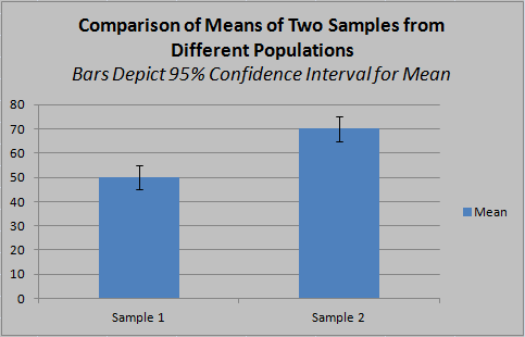
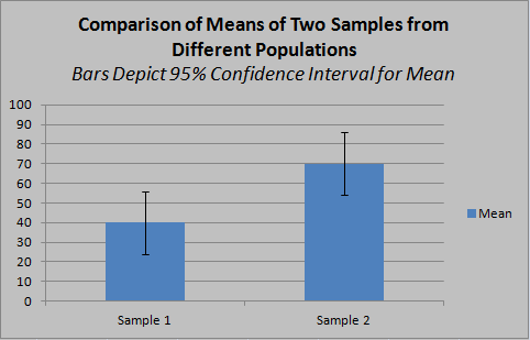
In the first example, the difference in means is statistically significant with a 95% confidence level, as the confidence intervals do not overlap. This means that, given the null hypothesis, random samples (of the same sizes as 1 and 2) would be expected to show at least this much difference in mean with a probability of 5% or less. In the second example, the measured difference in means, though greater in absolute terms, is not statistically significant (at the 95% level), since the confidence intervals do overlap. This means that, given the null hypothesis, random samples (of the same sizes as 1 and 2), there is a greater than 5% chance of observing a difference in means at least this large, so the null hypothesis cannot be safely excluded at this confidence level. The larger confidence intervals are driven by smaller sample size, making it more likely that a sample mean is less representative of the true population mean.
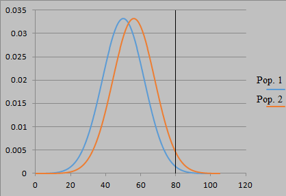
Naturally, one can statistically distinguish populations with true means that are less than a standard deviation apart, if the sample size N is large enough. Even small differences in the mean can lead to noticeably different proportions of values far from the mean. Below we depict two normal distributions of some variable, for which Population 1 has a mean value of 50 and standard deviation of 12, while Population 2 has a mean of 56 and standard deviation of 12. Although the separation of means is only 0.5σ, values of 80 or more are expected to be more than twice as frequent in Population 2 than in Population 1 (comparing the areas under the curves to the right of 80), an effect that we could surely detect with a sufficiently large sample.
If one population should have a larger variance or standard deviation than another, the disparity at extremes is more pronounced. Suppose Population 2 has a σ of 15 instead of 12:
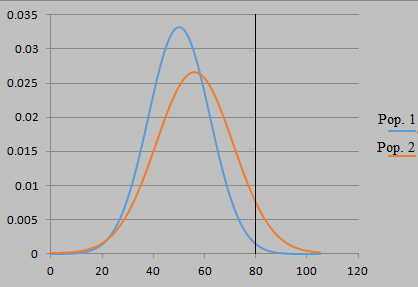
Far from reducing the detectability of differences, an increase in variance can make the difference in populations more readily detectable, as this larger disparity at extremes could be found with a smaller sample.
We should note that the validity of the t-test assumes homogeneity of variance, i.e., that the variances of the two groups are equal. In practice, however, the t-test works well even when the variances are unequal by a small ratio, as long as both samples have fairly equal numbers of subjects. Alternatively, an approximation known as the Welch t-test may be used for unequal variances. Using the t-test when the distribution is non-normal or the samples of unequal variances are also unbalanced in number will result in an overestimation of the level of confidence. What we call a 95% confidence interval may actually be only a 90% confidence interval.
In biological sciences, the confidence is expressed inversely in terms of the calculated probability that the results are consistent with the null hypothesis. When the t-test or ANOVA is used, this p value is effectively the complement of the confidence level, so p < 0.05 means a 95% confidence level. Analysis of variance or ANOVA is a generalization of the t-test to more than two groups. In place of N - 1, we use N - k, where k is the number of groups being sampled, to produce a less-biased (though not unbiased) estimator of the variance. The quantity N - k is called the degrees of freedom, i.e., the number of different ways the contributing values to the statistic could vary. (This should not be confused with the usage in physics and chemistry, where degrees of freedom
refers primarily to independent parameters contributing to a state, even in non-statistical contexts.)
The p values used in biomedical science literature are often misinterpreted. A p value of 0.05 does not mean that there is a 95% probability that the null hypothesis is false. The application of a statistical test requires us to assume that particular kinds of distributions would result if the null hypothesis or alternative hypothesis were true. This modeling of both hypotheses is assumed even when we are only testing the null hypothesis. A positive finding on our statistical test (i.e., excluding the null hypothesis at 95% confidence) means that it would be highly unusual (only 5% probability) to get such a large difference in sample means if the null hypothesis were true and all our modeling assumptions are correct (normal distributions, etc.). Also implicit are assumptions about the conduct of the analysis. If the protocol was violated, so that the two sample groups do not really reflect two distinct conditions, then the model is not applicable. If you conduct multiple experiments, and cherry-pick the one that gives you a small p, you have invalidated the probabilistic analysis by introducing a method of selection that is biased to favor a hypothesis.[9]
In short, statistical significance has to do with how confident we are that our difference in sample means reflects a real difference in means for the populations sampled, or more exactly, that there is a low probability that we could obtain our result accidentally by random sampling under the null hypothesis, given certain assumptions about the expected probability distributions under the null and alternative hypotheses. It does not indicate, on its own, the magnitude of the difference between the two populations.
Effect size,
distinct from statistical significance, measures the strength of correlation between two variables. When the two variables can each have many values, effect size is measured by the so-called correlation coefficient r (to be discussed in section 2.6). If we are comparing the same variable in two populations, we may treat membership in one or the other population as a second variable with two possible values. An estimator of the effect size in this scenario is Cohen’s d, which is defined as the difference in sample means divided by the pooled standard deviation. It is an attempt to measure how different two populations are, in terms of how non-overlapping their distributions are. Often, one of these populations is a control group, while the other is subjected to some experimental intervention, so the disparity ostensibly measures the magnitude of the intervention’s effect.
The pooled standard deviation is obtained not by treating the two sample groups as a single group for which we compute a standard deviation, but instead by taking a sort of average of the standard deviation in both groups:
spooled = √(Ne - 1)se2 + (Nc - 1)sc2/(Ne + Nc - 2)
Ne and Nc are the sample sizes of the experimental and control groups respectively, and similar notation is used for the standard deviations se and sc for each sample group. Cohen’s d is actually a biased estimator of effect size, overvaluing effect sizes (due to underestimation of the standard deviation) when sample numbers are small. This difference becomes negligble, however, for N > 50.[10]
Cohen’s d is |μe - μc|/spooled. By the symmetry of the formula, we could use it to measure effect size between any two groups, not just experimental versus control. Cohen himself offered the following standards for classifying effect sizes:
Standardized Mean Difference (Cohen’s d): Small = .20, Medium = .50, Large = .80
Correlation Coefficient (Pearson’s r): Small = .1, Medium = .3, Large = .5[11]
Since the comparison of means between two groups is just a special kind of bivariate correlation, every Cohen’s d can be converted into a correlation coefficient r = d/√d2 + 4. The value of computing an effect size is that it enables one to compare findings across studies that may use different measurement scales or units (as is often the case in psychology).
Cohen’s evaluation of effect sizes as small, medium or large was grounded in the context of psychology studies, and may not have the same significance in other sciences. A correlation coefficient of .5 would be considered a very weak correlation if one were a physicist testing for a linear relationship between mechanical variables. Cohen’s judgment that small
effect sizes are unimportant, regardless of statistical significance, is somewhat subjective and context-dependent. At most it means the two variables are not strongly correlated. In the case where one of the variables is membership in one or another group, it means that the distributions of values for a measured variable in each group are similar, i.e., mostly overlapping. We have seen, however, in the previous section that there could still be large differences in the extremes even when two distributions are mostly overlapping. The unimportance of small effects applies only to the populations in aggregate, and only to the means. We might have a small effect size where the means are just a fraction of a standard deviation apart, so that just 59% of the experiment group scores above the median score for the control group, but there could nonetheless be much larger differences in proportion at the extremes.
Effect size gives a good measure of how different two distributions are, but it does not necessarily tell us much about significance or importance, without introducing additional assumptions specific to a field of research or a particular kind of study. A difference in means with small effect size might still have important implications in cases where differences at the extremes are important. For example, two populations with slightly different mean intelligence, but much different variances, could differ greatly at the extremes. Despite the small
effect size for the mean, we would find a large disparity at the upper end of the intelligence spectrum. These high performers, though numerically small, may be of greater importance in terms of their impact on society.
Effect sizes can also be used for reverse calculations, for scientists to determine in advance how large a sample is needed in order to test for a medium
or large
effect. Smaller effects require bigger samples in order to be detected.
Significant effect size,
when applied to comparisons between groups, means that the distributions are mostly non-overlapping. This should not be confused with statistical significance,
which means that the measured difference in means, whether large or small in proportion to the pooled standard deviation, is unlikely to be the result of a random sampling error, and therefore may reflect a real difference in the underlying populations. The reality of the difference (statistical significance) is not abolished by its smallness in proportion to the distribution spread (small effect size). Significance
in statistical significance
means likely to measure a real difference in populations, insofar as it is not just an accident of sampling error. Significant
in significant effect size
means not small
in the sense of a non-small ratio of the difference in mean to the spread in distribution. On a practical level, you are determining whether a proposed intervention would have a small or large effect on the population as a whole. As we have noted, even a small effect on a population as a whole might be a great effect at the extremes.
Significance
is not necessarily the same as importance.
Consider an IQ study sampling two populations that gives means that differ by 3 IQ points and a pooled standard deviation of 6. Then consider another study sampling two different populations with means that differ by 5 IQ points and an spooled of 10. Both studies have the same effect size of .5, which would be a valuable comparison if each study was testing the same intervention to improve IQ. If they are purely observational studies, however, of different populations, then significance
is not necessarily the same as importance, as a 5 IQ point difference may be more important than a difference of 3. Yet even this is problematic, unless we have an understanding of what is being measured. Is a 5 point difference in IQ really measuring 160% as much difference in intelligence as 3 points difference? Or are differences meaningful only for 10, 20, or 30 IQ points? The judgment that an effect is significant does not necessarily tell us anything of its importance, without making judgments about the variable being measured.
An oft-repeated fallacy is that if variation within groups for some variable is greater than variation between groups, the latter variation is negligible or can be ignored. This is to mistake significance of effect size for statistical signifcance. The latter suffices to establish the probable reality of this finding of difference, regardless of the effect size. We must also keep in mind that Cohen’s definitions of effect size magnitudes were intended for psychology. In biology, even small
effect sizes can be physically meaningful changes, affecting major outcomes for an organism.
This fallacy is a misapplication of a statistical principle regarding resolution. Suppose you have two peaks in a multi-channel analyzer, which gives a histogram of various radiation frequencies. If the distance between the centers of the two peaks is less than the width of each peak, then you can not resolve the two peaks. In other words, you cannot be sure that you are really observing two distinct phenomena. Yet when we are measuring attributes of known groups, this limitation does not apply. We already know from other objective criteria how to distinguish or resolve the groups, so we can be sure we are observing two different distributions of the variable, even if the difference in mean is less than the standard deviation. Otherwise, we should absurdly have to claim that differences in mean between populations less than a standard deviation is never possible, since we could never observe it even if we measured both entire populations.
The above discussion assumes we are dealing with fixed effects,
i.e., we are systematically changing a variable (either by sample selection or by intervention) for one or another group, so our measured effect size ostensibly is a result of this fixed change. In reality, however, research on human subjects often involves effectively random factors (unobserved heterogeneity) that can’t be modeled as a fixed parameter. If we conduct an IQ study across various schools to test whether a certain model of education affects outcome, we must also account for the innumerable random (i.e., unpredictable or unidentifiable) differences due to the individual competences of teachers and administrators. This is done by introducing random variables as model parameters. In biostatistics, subject-specific effects are often characterized as random,
because in practice we cannot account for all the innumerable differences between individuals and select for them. Nonetheless, there are contexts where we may try to understand inter-individual differences by fixed effects, selecting or classifying subjects by certain genetic or biochemical markers. Fixed
and random
here mean correlated and uncorrelated to the independent variable(s) (outcomes) under investigation.
If we are modeling two or more effects—one fixed and one random; two fixed; two random, etc.—we must use a multivariate measure of effect size, such as Cohen’s f2, which will have different values for small,
medium,
or large
effect sizes. There are many measures of effect size besides Cohen’s, though his are most widely used. If there is at least one fixed effect and one random effect modeled, this is known as mixed-model
analysis. Generally, mixed model analysis is necessary only when sampling from many groups that are likely characterized by some unmeasurable (under the current protocol) variable(s) that may affect the outcome(s) being measured. It becomes less necessary insofar as our sampling is truly randomized for individual differences in a population, without selecting clusters of subjects in different groups characterized by unmeasured yet relevant variables.
Statistical measures such as mean and variance may describe the distribution of a property in a population, without telling us anything about what causes it to be so distributed. A necessary (but not sufficient) condition of causation is that there should be some correlation between a cause and its effect, i.e., where the purported cause is present, the effect is at least more likely to occur. Thus a study of correlations is a valuable precursor to the discovery of causes. To determine empirically if two properties, characterized by the variables X and Y, are correlated, we must measure the values of these properties in many individuals, and see if X generally increases or decreases when Y increases or decreases. The presence of some statistical correlation need not imply absoluteness. It is not necessary that every individual with a higher value of X should have a higher value of Y; the correlation in X and Y values may merely hold for most members of the population.
A correlation coefficient, with values ranging from -1 to 1, measures how strongly correlated two variables are. A positive value means that when one variable tends to increase when the other increases, and a negative value means one variable tends to increase when the other decreases. The greater the magnitude of the value, the more strongly correlated the two values are, with a magnitude of 1 signifying linear proportion. Thus a correlation coefficient may also be considered a measure of how well the data can be fitted to a line. A more exact construction of the correlation coefficient follows.
The mathematical expectation or expected value (expectation value
in physics) of a random variable is a probability-weighted average of all possible values for that variable. For a discrete variable X, E(X) = ∑pixi, where pi is the probability of the possible value xi, and ∑ represents the sum over all different possibilities represented by values of the index i. If X is a continuous variable, E(X) = ∫xp(x)dx, where p(x) is the probability density function of X. Note that the expected value, being a probability-weighted average, need not correspond to an especially probable or even possible value of X, just as an arithmetic average of values need not be identical with any particular value, so expected value
is a bit of a misnomer. The expected value need not coincide with the median or midpoint of the distribution where half the probability is above or below it, though this is the case for a normal distribution. Rather, the expected value is the long-term average value of the variable that we should expect if we could acquire an arbitrarily large number of data points.
The covariance of two variables is the expected value (probability-weighted average) of the product of distances from the mean for each variable.
Cov(XY) = E[(X - μX)(Y - μY)]
The covariance is sometimes denoted σXY, though this can wrongly suggest it is a kind of standard deviation. The only way a covariance is even definable is if there are data points that have values for both variables. For that population, we take each individual’s values for X and Y, compute the distance from the mean for each value, take the product, and then sum over all possible X-Y value combinations, weighted for probability, and dividing by N, the size of the population.
If X and Y are discrete variables, and all values of each variable are equiprobable, the covariance is:
Cov(XY) = (1/N)∑(xi - μX)(yi - μY)]
where i ranges from 1 to N.
If X and Y are positively correlated in a given population, we should expect a statistical correlation in X and Y values. If an individual has a value for X above the mean of X, we should expect it, on average, to have a value for Y above the mean for Y. The further above the mean its X value is, so its Y value should be proportionately further above the mean for Y. Again, this should hold on average, if not in every or even most particular instances.
Usually we cannot know the true mean of a population, so we cannot know the true covariance of the population. Instead we use the sample covariance as an estimator. As with the sample variance, we must divide by N - 1 instead of N. If values are not equiprobable, just multiply by N/(N - 1).
The correlation coefficient rXY is the covariance divided by the product of standard deviations.
rXY = Cov(XY)/σXσY
Correlation coefficients thus normalized may have values ranging from -1 to 1. If we are dealing with random samples, we must first divide each product of distances from the mean by the sample standard deviations, then take the sum over all data points, and divide by N - 1.
rXY = ∑(xi - μX)(yi - μY)/sXsY(N - 1)
Here r is the sample correlation coefficient, s is the sample standard deviation (using N - 1) and μ is the sample mean.
By expressing correlation as a ratio of covariance to standard deviations, we say that correlation is stronger for a given covariance if the standard deviations or spread is smaller. Strength of correlation is indicated by the absolute value of r, with a minus sign meaning negative correlation (i.e. one variable increases as the other decreases). A perfect correlation of ±1 would mean the covariance is equal in magnitude to the product of standard deviations, as it cannot be greater. 100% correlation would mean X always increases (or always decreases) with Y for all individuals and proportionately.
Even with strong or perfect correlation, we have not established causality, though it is strongly suggestive of a causal relation, since we do not believe that such things can be mere happenstance. (Indeed, there are statistical tests to estimate the probability of this happening randomly, based on the number of individuals measured.) It is a philosophical assumption, though one essential to science, that non-random correlations of physical quantities are to be accounted for by some physical cause. Even granting this assumption, we cannot immediately discern what is the cause and what is the effect. Supposing that variables X and Y are strongly correlated, it is possible that (a) changes in the property described by X cause changes in the property described by Y; (b) changes in Y cause changes in X; (c) some common factor Z causes changes in both X and Y, so that neither X is the cause of Y nor Y of X.
Interpreting correlation coefficient values in terms of physical significance depends on context. r = 0.5 would be a dismally low coefficient in most physics contexts, as it would show that there is not a strong linear relation, so some other model of dependence is needed. In biomedical sciences, this may be considered a strong finding of dependence, since we have no expectation of strongly deterministic correlations approaching 1 in complex organisms with many confounding factors of disparate conditions (unlike in physics, where one can often control conditions to make particles practically identical in description). As always, statistical outcomes such as correlations are only as good as the data quality. If the protocol for intervention and control subjects is not consistently applied, or there is some systematic error, we could find false correlations or fail to find those that do exist.
In experimental contexts, one of the variables, say Y, is deliberately controlled (by intervention or by selection of subjects) in order to ascertain if there is any effect on the other variable X. In this situation, Y is called the independent variable, while X is the dependent variable. Although we speak of effect,
in fact we are only testing for correlation, a necessary but not sufficient condition of causality.
If we want to test the effects on X of two or more independent variables, we must use multiple correlations among the three or more variables, and construct a multiple correlation coefficient from the correlation coefficients of each pair of variables. The full generalization involves matrix and vector algebra.
We have mentioned that a comparison of means is a special case of bivariate correlation, so for every Cohen’s d we can compute a correlation coefficient. Likewise Cohen’s f2 is a special case of multivariate correlation.
The mere computation of correlation coefficients does not tell us the specifics of the correlation, i.e., the slope and intercept of the line that best characterizes the relationship between variables. This is achieved by simple or multiple linear regression, for two or more variables.
Multiple effect variables may be classified hierarchically in what is called a multilevel model. Each level is assumed to have a linear relationship, but the parameters of each level (slope and intercept) are allowed to vary linearly according to the higher level variables. For example, we could treat household income as a Level 1 predictor of math achievement, and school district as a random-effect Level 2 predictor, thereby allowing that the correlation parameters (slope and intercept) between achievement and income may be different in each school district, owing to the unique factors of each school system or its neighborhood. School district may be treated as a random
parameter insofar as it is uncorrelated to the independent variables measured (in this case income), though it may nonetheless contribute to the outcome variable (achievement).
One benefit of multilevel modeling, though not its primary purpose, is that we can compute within-cluster
correlations as (s2Ts2C)/s2T, where s2T is the total variance across all clusters, while s2C is the variance within a cluster, say a school district. If the variance within a cluster is much smaller than the overall variance, this indicates that the dependent variable is indeed affected by being in a particular cluster. If, on the other hand, the within-cluster variance is about the same as the overall variance, then the within-cluster correlation is close to zero.
Multilevel modeling can be valid and useful only if we are dealing with a large number of groups or clusters (30, 50 or more). Otherwise we might actually be introducing bias by choosing to cluster our data.
We have assumed so far that correlations are linear, but regression modeling can be generalized to logarithmic correlations. For other non-linear correlations, such as higher order polynomials and trigonometric functions, we may use other kinds of regression or the chi-squared statistic to measure the goodness of fit for multiple parameters. The latter is used mainly in physics, where there is a theoretical basis for expecting more sophisticated mathematical correlations. In biology, observed correlations are often too messy to be described more precisely than by approximate linear proportion or logarithmic correlation. If there is an unknown multi-parameter correlation underlying a phenomenon, this could be missed by linear regression analysis, giving a misleading result of weak correlation.
In biomedical studies, there are countless measuring tools such as surveys and cognitive tests, each of which can have many outcome variables (e.g., responses to particular questions, scores on a subsection or overall test). These measured variables may be correlated to each other in a way that can be characterized by a fewer number of underlying variables. The observed variables, being the outcomes of artificially designed tests, are thought to reflect some real underlying biological or psychological abilities, to which the underlying variables may correspond. For example, doing well on test A may correlate strongly to doing well on test B, but performance on A and on B are both uncorrelated to performance on test C. Thus performance on tests A, B and C might be well characterized by just two variables instead of three. The number of underlying variables are the degrees of freedom or dimensionality of the system, and each variable may be considered a potential causal factor, or at least a correlative factor. All the observed variables may be represented as linear combinations of the underlying variables, and the correlations among observed variables are explainable in terms of correlations among the underlying variables.
Charles Spearman developed factor analysis in 1904, in order to show that the specific intelligences
measured by various tests in the classics, English, mathematics and other subjects were all strongly correlated to each other and to a single general intelligence
factor. After properly accounting for the different metrics and irrelevant factors, the variance of results on each test could best be explained by a two-factor model, one factor being general intelligence
and the other factor being specific to that test.
An exposition of factor analysis[12] requires principles of multivariate correlation that we have so far discussed only briefly. When we have three or more variables, it is useful to know all covariances and correlation coefficients between every pair of variables, and to order these in a matrix for analysis. Mere inspection of these correlations is often insufficient, especially for many variables, as analysis may show that they are interrelated in subtle ways. It need not be simply that variables A and B are correlated and C and D are correlated. Rather, A, B and C may be correlated to some underlying variable E, while C and D are correlated to another underlying variable F.
Suppose some variable Y can be expressed as a linear combination of the variables Xi.
Y = c1X1 + c2X2 + c3X1…
Y = ∑iciXi
The mean of Y is simply the same linear combination of the means:
μY = ∑iciμXi
The variance of Y is a double sum over all possible pairings of variables (counting non-identical pairs twice) of that pair’s covariance times the coefficients for that pair:
σ2Y = ∑j∑kcjckCov(XjXk)
When j = k, that self-pairing is only counted once and the covariance
is really just the variance of that single variable. This formula is for population variance, which is unknowable (unless the entire population is measured), though sample variance may be used as an estimator.
Suppose there are two variables, Y1 and Y2, each of which is a linear combination of Xi.
Y1 = ∑iciXi
Y2 = ∑idiXi
Then the correlation between Y1 and Y2 is given by the usual formula:
rY1Y2 = Cov(Y1Y2)/σY1σY2
In order to perform multivariate analysis, we should first make sure that each of our variables Xi has a normal distribution. If this is not the case, we can try taking roots or logarithms of our data in order to obtain approximately symmetric normal distribution, and then use this modified function, e.g. X1/2, log10(X) as our variable instead. In what follows, we assume that all Xi have normal distributions.
In a multivariate model, each variable X takes vector values instead of simple numeric (scalar) values. We may express X as X = (X1, X2, X3…), where the elements Xi are independent variables. For example, suppose a population of students takes three tests A, B and C. Their scores on this set of tests may be expressed as X = (A, B, C), where A, B and C are normally distributed random variables.
It is computationally useful to have in hand a matrix of covariances among independent variables, which we show in tabular form:
| A | B | C | |
| A | σ2A | Cov(AB) | Cov(AC) |
| B | Cov(BA) | σ2B | Cov(BC) |
| C | Cov(CA) | Cov(CB) | σ2C |
The diagonal elements are just the variances of each variable, and the matrix is symmetric since Cov(AB) = Cov(BA). We could convert this into a table of correlation coefficients among variables by multiplying by the product of standard deviations for each variable pair. This would give a value of 1 for diagonal elements:
| A | B | C | |
| A | 1 | rAB | rAC |
| B | rAB | 1 | rBC |
| C | rAC | rBC | 1 |
The square of the correlation coefficient, known as the coefficient of determination, tells us what percent of the variance for a given variable is correlated to each other variable.
The covariance matrix can be subjected to the usual analysis of linear algebra. The trace or sum of its diagonal elements is known as the total variation, since it is the sum of the variances of all variables. The determinant of the covariance matrix is called the generalized variance. In practice, we use the determinant of the sample covariance matrix as an estimator for the population.
Let Σ represent the covariance matrix, and |Σ| is the determinant of that matrix. Then the probability density function φ of a random vector X with a multivariate normal distribution is given as:
φ(X) = (1/2π)n/2|Σ|-1/2exp{-(1/2)(X - μ)T∑-1(X - μ)}
where n is the number of coordinates in X (i.e., the number of random variables), μ is the mean vector (whose coordinates are the mean of each variable), and T signifies the transpose of the column vector, i.e., a row vector. When n = 1, we have a univariate distribution with a bell curve in two dimensions. When n = 2, we have a bivariate distribution with a bell curve in three dimensions, and so on.
The factor (X - μ)TΣ-1(X - μ), known as the Mahalanobis distance, gives a sort of generalized distance between x and μ, taking the variances into account in order to weight the significance of deviations from the means. The Mahalanobis distance squared has a chi-squared distribution with n degrees of freedom. Thus the probability of the Mahalanobis distance being less than or equal to χ2n, α is 1 - α. We usually choose α = 0.05, for 95% probability.
The Mahalanobis distance has the algebraic form of a hyper-ellipse in n-dimensional space centered at μ. The axes of the ellipse are oriented along the eigenvectors of the covariance matrix, and the length of each semi-axis is given by √λiχ2n, α, where λi is the eigenvalue for the ith eigenvector. If α = 0.05, then there is a 95% probability that a random value of X will fall within the ellipse.
If two variables are uncorrelated, so r = 0, the eigenvalues will be the variances σ12 and σ22. The ellipse
will just be a circle. For strongly correlated variables, as r approaches 1, the two eigenvalues will approach σ12 + σ22 and 0, and the ellipse will become eccentric and approximate a line segment at a 45-degree angle.
We may think of the variable defined along each eigenvector as accounting for a share of the total variance, the magnitude of this share being measured by the eigenvalue. When we have many random variables with complicated correlations, we should like to identify systematically a set of eigenvectors such that each one, in order, accounts for the largest possible share of the variance. Such a procedure is known as principal component analysis (PCA).
In PCA, the desired principal components are assumed to be linear combinations of the random data variables X = (X1, X2, X3…), so that these principal components likewise constitute an array of random variables Y = (Y1, Y2, Y3…).
Y1 = e11X1 + e12X2 + … + e1rXr
Y2 = e21X1 + e22X2 + … + e2rXr
…
Yr = er1X1 + er2X2 + … + e1rXrr
More succinctly, this can be expressed as:
Y = EX
where Y and X are column vectors, and E is the r × r square matrix consisting of the components eij. We may subdivide this matrix into column vectors denoted ei = (ei1, ei2… eir).
The variance and covariances of the principal components are:
Var(Yi) = ∑k,l eikeilσkl = eiTΣei
Cov(Yi, Yj) = ∑k,l eikejlσkl = eiTΣej
where Σ (without indices) is the covariance matrix of X and eiT is the row vector or transpose of ei.
To find the first principal component Y1, we must choose coefficients e1j that maximize the variance of Y1, so it accounts for as much of the total variance as possible. The vector e1j will be an eigenvector of Σ corresponding to the largest eigenvalue of Σ. By convention, the sum of the squares of e1j is required to be 1, so the vector e1j is of unit length. Since scalar multiples of eigenvectors point in the same direction and correspond to the same eigenvalue, there is no loss in generality.
For the second principal component Y2, we must find the coefficients e2j that maximize the variance of Y2, while at the same time making Y2 completely uncorrelated to Y1, so they do not account for overlapping shares of the variance. That is, Cov(Y1, Y2) = 0. These coefficients will form the eigenvector of Σ corresponding to the second largest eigenvalue of Σ.
Each successive principal component is subject to similar constraints, with the added condition that it must be completely uncorrelated to all previous principal components.
Since there can be fewer than r eigenvalues in an r × r matrix, there may in general be fewer principal components than data variables Xi. The fraction of the variance accounted by each principal component Yi will be its corresponding eigenvalue λi divided by the sum of all eigenvalues of Σ.
Although the formal results above apply only to the unknown true
covariance matrix Σ, in practice we can use the sample covariance matrix as an estimator. To avoid making our analysis dependent on the choice of units for each variable, we may standardize the variables, replacing the Xi with the standardized Zi:
Zi = (Xi - μ(Xi))/σi
We divide the difference in values from the mean by the standard deviation. Since we work only with the sample data, we must use the sample standard deviation instead of the ideal σi. This standardization, however, changes the covariance matrix, so the covariance matrix of Z equals the correlation matrix of the raw variables X. Thus, if we are standardizing variables, we must instead use the matrix of correlation coefficients of the original variables X, rather than the covariance matrix.
Factor analysis itself is an inversion of PCA. We model the observed variables Xi as a linear combination of unobserved factors.
(Since the factors are unobservable, we cannot actually check for linearity.)
Xi = μi + li1f1 + li2f2 + … + limfm + εi
The data from each individual subject may be expressed as a column vector of observed variables or traits: X = (X1, X2, …, Xr). The population means μi of the observed variables are also expressible as a column vector, and may be considered the intercepts of the linear regressions. The coefficients lij, known as factor loadings, can be represented as an r × m matrix, where the number of factors m is generally less than the number of trait variables r.
X1 = μ1 + l11f1 + l12f2 + … + l1mfm + ε1
X2 = μ2 + l21f1 + l22f2 + … + l2mfm + ε2
…
Xr = μr + lr1f1 + lr2f2 + … + lrmfm + εr
The system of equations can be expressed in terms of the matrix of factor loadings L as:
X = μ + Lf + ε
The column vector of factors f has only m components, but left multiplication by L yields a vector of r components. The random error terms εi are called specific factors, for they may be considered factors that are specific to one observed variable and uncorrelated to all other variables.
In order to arrive at a unique set of parameters l, f, ε, the following conventional assumptions are introduced. The mean of each error εi and each factor fi is assumed to be zero. Thus we define the mean response of each observed trait Xi to be simply the population mean μi. The variance of each factor fi is assumed to be 1, as is Var(εi), the specific variance. The common factors fi and specific factors εi are all uncorrelated with each other, so we are only looking for independent factors.
With these assumptions, the variance of each trait i is:
Var(Xi) = ∑j lij2ljk + Var(εi), where where j = 1, 2,…m
The covariance between two traits is:
Cov(Xi, Xj) = ∑k likljk, where k = 1, 2,…m
The covariance between a trait and a factor is equal to the factor loading.
Cov(Xi, fj) = lij
The sum of the squares of factor loadings lij for a given trait i is known as the communality, a measure of how well the model performs for that trait.
The covariance matrix Σ is:
Σ = LLT + Ψ
where Ψ is the matrix of specific variances. Its diagonal elements ψi are the specific variances, and its off-diagonal elements are zero.
Factor analysis entails estimating the parameters of a linear model for a set of factors, i.e., estimating the factor loadings lij and the specific variances ψi.
There are several methods of factor analysis. Under the principal component method, we use the eigenvalues and unit eigenvectors of the matrix of sample covariances (with a divisor of N - 1 instead of N) as estimators. The index i in the expressions below designates the row of that matrix, i.e., it indexes the observed variables Xi. The index j corresponds to a column of that matrix, i.e., indexing the factors fj.
lij = eji√λj
ψi = si2 - ∑j λjeji2
Since the entire point of factor analysis is to see if we can explain our observed variables in terms of a fewer number of factors, we only sum from j = 1 to m, the number of factors. eji means the jth component of the ith eigenvector. The us the second equation means that the specific variance equals the sample varaince minus the communality.
We can attempt factor analysis with different numbers of factors, to see what percent of the variation can be explained by so many factors. We use the first equation to calculate estimated factor loadings, which are correlation coefficients between the factors and the variables. We can thus think of the factor loading matrix L as a correlation matrix. From that matrix we can calculate communalities by taking the sum of squares of factor loadings for a variable Xi:
hi2 = ∑j lij2
The sum of the communalities for all variables divided by the number of variables gives the percent of variation explained by the model.
Although factor analysis is useful for telling us how mnay factors there are, it cannot tell us unambiguously what the factors are. Suppose we have a survey with five questions A-E, each of which asks for an answer on a scale of 1-10. We have five observable variables, A-E. After testing many subjects, we find that answers to some questions are more strongly correlated than others. We may find that, assuming that there are only two underlying variables, we can account for 70%-80% of variance. Thus we may have good cause to think that two variables suffice, since the remaining unaccounted variance may be due to the limitations of methodology or sampling in biomedical science. This does not uniquely specify what those variables are, however. One variable could be in the space spanned by A, B, and C, and another could be in the space spanned by D and E, but this does not tell us anything more specific.
The number of factors describing the variance is a number of independent variables, which is not to be confused with the number of parameters in a fit between two variables. For the latter, a linear fit has two parameters (slope and intercept), a quadratic fit has three parameters, and so on. In factor analysis, each factor is an independent variable, supposed to be correlated to other factors linearly (i.e., by two parameters).
Analysis of variance (ANOVA) is a two-way factor analysis, testing the equality of the mean in two groups. It is useful when you do not care about the true value of the mean, but only wish to explain the variance. The variance in each group may be better explained on the assumption of a single factor (i.e., the observed variable, with group difference being negligible), or on the assumption of two factors (with choice of group being the second factor).
The exact methodology of factor analysis, judging when to include or exclude an additional factor, is not without controversy. Often the standards or thresholds vary by particular fields, such as psychometrics, when one is trying to determine how many factors can explain intelligence or personality.
Even with the model assumptions described earlier, the solutions of factor analysis are not unique for a given number of factors. A factor loading matrix that is a rotation
of L will also be a solution. Sometimes we want to seek out a rotation that will make each factor correlate strongly to a fewer number of observed variables, on the grounds that this is more parsimonious and more likely to reflect a truly causal account of the observed variables. This too is a disputable subjective judgment. So, for all its mathematical complexity, factor analysis is of limited utility for ascertaining the true
variables underlying what we observe, though it is at least reliable for ascertaining the dimensionality or number of degrees of freedom that account for most of the variance. Even here we should note that factor analysis ignores any variance not counted in the correlation coefficents.
Continue to Part III
[5] This way of speaking about selecting advantageous traits should not be construed as implying anything purposive or deliberate in the evolutionary process itself, but rather the outcome of a stochastic process. On the other hand, this does not preclude theism as understood by Aristotle: nature is not divine, though it is divinely ordered. In other words, there is no intelligence in natural processes themselves, but in the cosmic order that makes such processes possible.
[6] In fact, case-based reasoning
has been shown to have a quantifiable probabilistic value, justifying its application in medicine and other fields. See: Begum, S., Ahmed M.U., Funk, P.; Xiong N., and Folke, M. Case-Based Reasoning Systems in the Health Sciences: A Survey of Recent Trends and Developments.
IEEE Transactions on Systems, Man, and Cybernetics, Part C: Applications and Reviews. July 2011. 41(4): 421–434. doi:10.1109/TSMCC.2010.2071862
[7] As of June 2017.
[8] R. Hogg and E. Tanis. Probability and Statistical Inference, 5th ed. (Upper Saddle River, NJ: Prentice Hall, 1997), pp.282-298.
[9] For further discussion, see: S. Greenland et al.. Statistical tests, P values, confidence intervals and power: a guide to misinterpretations.
European Journal of Epidemiology. 2016. 31:337-350.
[10] L.V. Hedges and I. Olkin. Statistical Methods for Meta-Analysis (Orlando, FL: Academic Press, 1985). For smaller N, one may use Hedge’s correction factor, which uses the gamma function. L.V. Hedges. Distribution theory for Glass’s estimator of effect size and related estimators.
Journal of Educational Statistics. 1981. 6(2): 107-128. doi:10.2307/1164588
[11] Jacob Cohen. Statistical Power Analysis for the Behavioral Sciences (1988). The category Very Large
for d = 1.30 and r = .7 was added by Rosenthal (1999).
[12] This presentation of multivariate, principal component and factor analysis follows the mathematical content of the online course materials for STAT 505: Applied Multivariate Statistical Analysis, (Pennsylvania State University, 2021, licensed under CC BY-NC 4.0), with some minor changes in notation and some added exposition of concepts.
© 2021 Daniel J. Castellano. All rights reserved. http://www.arcaneknowledge.org
| Home | Top |