


The St. Petersburg paradox is a problem in probability theory, first published in the Commentarii Academiae Scientiarum Imperialis Petropolitanae by Daniel Bernoulli in 1738, in which the mathematical expectation or probability-weighted payoff of a hypothetical game is infinite due to geometric increase of progressively improbable payoffs. As early probabilists believed that the fair cost of entering a game ought to equal the mathematical expectation, this presented a perplexing contradiction, as no reasonable player should wager an infinite sum on this game, if that were even possible, since the probability of an infinite payoff is zero. Probability theory arose as a form of mixed mathematics
that applied mathematics to practical problems of contract equity, so this disparity with intuitive notions of reasonableness and fairness was considered a real failing.[1]
The hypothetical game, first formulated by Bernoulli’s cousin Nicolas privately in 1713, consisted of a series of coin tosses, which ended upon the first toss of heads. If heads appeared on the first toss, the player received one ducat. The payout was two ducats if heads first appeared on the second toss, four ducats if on the third toss, and so on, doubling each time. The probability of winning one ducat was 1/2, of winning 2 ducats was 1/4, of winning 4 ducats was 1/8, and so on. The mathematical expectation is thus (1/2) × 1 + (1/4) × 2 + (1/8) × 4 + … = 1/2 + 1/2 + 1/2 + …, which is infinite. If, as was commonly reckoned, the value of the opportunity to play a game is its mathematical expectation, then the value of playing this game should be infinite. Yet a reasonable man might gladly sell his opportunity to play this game for 20 ducats or less.
The St. Petersburg paradox is not a true paradox as far as mathematics or probability is concerned. The mathematical result of an infinite expectation is unequivocal and correct. What is unusual about the St. Petersburg game is that most contributions to this expectation are loaded into progressively low probability events. This somehow generates a disparity between mathematical expectation and real-world expectation regarding the game’s payoff and thus its value to the player.
To account for this disparity between mathematical expectation and how most men would value such a game, Daniel Bernoulli himself proposed a measure of utility distinct from mathematical expectation, grounding this in the finite wealth of a player, so that retaining an amount has utility in proportion to its fraction of the player’s total wealth. He expresses this in infinitesimal increments dx/x, from which integration yields a natural logarithm. Thus it may be considered a log utility function, such as is used by some modern economists in decision theory. This logarithmic utility rate offsets the exponential growth of stakes for low probability events, rendering the expectation finite, with a value dependent on the player’s total wealth. This moral expectation
is different from the mathematical expectation as it uses the utility function to arrive at a different valuation of payoffs versus the benefit of retaining one’s money.
The log utility function is not the only solution that would eliminate the infinite expectation. Gabriel Cranmer had earlier shown to Nicolas Bernoulli that a square root utility function would achieve this effect. He based diminishing utility on the notion that larger payouts would have smaller marginal utility as one progressed, i.e., once you have the possibility of winning a large sum, the smaller possibility of an even larger sum does not appreciably improve the game, for one only needs so much money.
Addressing the St. Petersburg problem was a practical imperative among all early probabilists. Most famously, Laplace accepted Daniel Bernoulli’s solution, using it to define a moral expectation
as a tenth fundamental principle of probability theory. In Laplace’s version, the stake on the first toss was 2 francs rather than 1 ducat, and doubled thereafter, so the mathematical expectation was 1/2 × 2 + 1/4 × 4 + 1/8 × 8 + … = 1 + 1 + 1 + …, which is still infinite. Laplace showed that Daniel Bernoulli’s solution had the advantage of reducing to the mathematical expectation as the changes due to playing the game were negligible compared to a player’s wealth, i.e., as a player’s initial wealth approached infinity.
Later commentators have addressed the problem by various approaches. Many have adopted one or another model of utility, showing how it deviates from mathematical expectation. However, it is always possible to make the stakes of the lottery increase faster than can be offset by any given utility function. Some, following Nicolas Bernoulli, believe that people simply disregard lower probability events, or offer some other psychological explanation for why they might undervalue such a game. These exercises in decision theory require us to dive deep into human psychology and economic circumstances, and Laplace himself admitted that it was impossible to account for all such contingencies.
The most insightful early solution, in our view, is that of G.L.L. Buffon (1777), for he recognized that the average payoff depends on the number of games played, so this should be factored into our expectation. If one plays a number of games equal to a power of 2, we can express as integers the expected number of games to end with the first toss, second toss, third toss, etc. We expect the game to end on the first toss half the time, on the second toss a quarter of the time, etc. Thus if we play 2s games, the first payoff may be expected 2s − 1 times, the second payoff 2s − 2 times, all the way to the sth payoff, which may be expected once. If, as Buffon claims, we can safely disregard the fact that this only adds to 2s − 1 games, then the expected payoff (if minimum payoff is 1) after 2s games is:
∑si=12s−i ⋅ 2i−1 = 2s ⋅ s/2
Thus the average payoff per game is s/2, i.e., it is explicitly a function of the number of games played! This is contrary to our ordinary probabilistic treatment of repeated games, where the expectation is independent of the number of games played. Sydney Lupton (1889) generalized this result to any number of games N, even if not a power of two. The average payoff will be (1/2)⋅log2N.
It is not enough to consider the mathematical expectation of a game when determining a reasonable stake. The cumulative payoff per play can be expected to approximate the expectation value only after a large number of trials, but the size of this number, or more precisely, the rate of convergence to the mean, varies by the design of each game, i.e., by its probability distribution. In the case of the St. Petersburg game, it is highly unlikely that any but the lowest payouts will be won even after hundreds of plays. Contrast this with other games such as roulette, where playing a given number can be expected to pay out after a few dozen tries. Even slot machines, the least favorable casino game, usually have several tenfold to twentyfold payouts and at least one mid-size (fifty- to eightyfold) payout after a few hundred plays. In short, a player has a realistic chance of cycling through most of the possible prizes in an evening. The question is whether he will win more than he loses, not whether he has a realistic chance of ever winning a sizable prize at all.
For low probability, high payout games, such as national lotteries, a player will only wager small amounts that he can afford to throw away. Odds generally do not figure into this decision making; in fact the odds of winning all but the largest jackpots are not worth even a one dollar wager. The purchase of a lottery ticket is made worthwhile only by virtue of smaller, more probable prizes, though even these have odds much less favorable than those offered by casinos.
The St. Petersburg game has a highly asymmetric distribution, so that most of the expectation value is generated by wildly low probability events. Since a player will only play a finite number of times, the odds of getting any of the larger payouts is much too negligible to be worth considering. We can quantify this more exactly by computing the probability of failing to get a certain level payout after a certain number of plays.
In the table shown below, we follow Laplace’s version of the game, where the payout is 2 francs if the first heads is on the first toss, 4 francs if it is on the second toss, 8 francs on the third, and so on. The mathematical expectation is 1 if we consider only the first payout as possible, 2 if we consider the first two payouts as possible, 3 for the first three payouts, and so on. We can easily calculate the probability of winning each payout in a single play, and the probability of failing to win that payout would just be 1 minus the probability of winning it. We take this probability of failure in a single game and multiply it by as many times as the game is played. This gives the probability of not winning that payout at all after that number of plays. 1 minus this amount is the probability of winning that payout at least once after that number of plays.
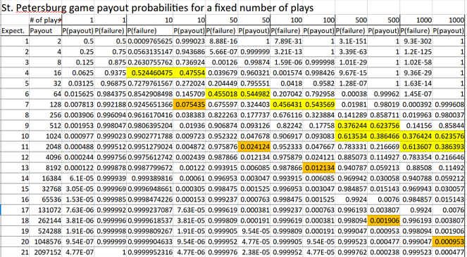
There are a couple of intuitive measures for determining whether a player should regard a payout as worth considering. One might only consider the payouts that one has about a 50 percent chance of winning at least once after a given number of plays. These figures are highlighted in yellow. By this measure, the player should only consider the first 4 payouts as likely to occur after 10 plays, and so should reckon the expectation only as 4 for the purpose of his limited play. We should note, however, that the 52 percent chance of failing to get the 16 franc payout applies only to that specific payout, and does not exclude higher payouts, which may still have significant probabilities less than 0.5. So this is a conservative measure or lower bound on what one might wager: 4 francs per game if one is to play 10 times, 6 francs per game for 50 plays, 7 francs per game for 100 plays, 9.5 francs per game for 500 plays, 10.5 francs per game for 1000 plays.
A better threshold (highlighted in orange) might be to consider any payout with a probability of at least 1/N where N is the number of plays. By this standard, we should bet 7 francs per game to play 10 times, 11 francs per game to play 50 times, 13 francs per game to play 100 times, 18 francs per game to play 100 times, and 20 francs per game to play 1000 times. These figures are much more in line with what others have proposed as reasonable. For these first two methods, we could interpolate the probability function to 0.5 or 1/N to provide more exact figures.
We might also apply Lupton’s generalization of Buffon’s payoff calculation in terms of number of games played. Doubling this payoff to follow the Laplace convention means the expected payoff is log2N. Accordingly the wager per game to be placed based on total number of games N is:
| N | Stake |
|---|---|
| 1 | 0 |
| 10 | 3.322 |
| 50 | 5.644 |
| 100 | 6.644 |
| 500 | 8.966 |
| 1000 | 9.966 |
Buffon’s approximation excludes everything above the sth payoff for 2s plays. If we play 1024 times, we should ignore everything above the possibility of 10 tails in a row. If we play 4 times, we should ignore everything above the possibility of 2 tails in a row. These exclusion thresholds are more subject to error for a smaller number of plays (and is absurd in the case of N = 1). When we get to larger N, especially N ≥ 100, however, these wagers track nicely with what we have identified as the 0.5 probability threshold for a particular outcome. We note, however, that the excluded possibilities have non-negligible probabilities. Buffon’s approximation assumes an idealized distribution of outcomes rather than a genuinely random distribution.
In no circumstance should a player be willing to wager an infinite sum, even if such a thing were possible to him, for then he is absolutely certain to lose more than he wins. The infinite expectation value can only be approached, never achieved, not even with a remote probability, in any play of the game, as the probability of an infinite chain of tails is zero, and a payout requires a heads, the attainment of which would make the chain of tails finite. Only an infinite number of plays would make the expectation approximate infinity, but infinity is not a number, but an unending succession. Even if a player had unlimited time, his winnings would never even approximate infinity at any point in time. Saying something takes an infinite amount of time (or number of plays) is the same as saying one will never attain it. To be sure, the longer the period of time or number of plays, the more payouts that can be taken into consideration and thus a higher expectation.
Back in the real world, no one is likely to wish to play the St. Petersburg game more than 1000 times, though that could be magnified if a computerized version were played. Regardless of what that limit is for players, we will have a contradiction of interests that makes the game impossible. Though each player, for example, will play no more than 1000 times, the house or casino will likely have many players, which will make the total number of plays much greater, bringing the higher payouts into play and causing losses to the house if they agree to a 20 francs stake that is reasonable for the 1000-game player. Unless the players are willing to stake much more, which would be highly unfavorable to them, no sensible casino will operate such a game.
The game could be modified to be made equitable to both parties. Since the players are only wagering based on payouts up to a certain limit, the house should not offer them the opportunity to play for those higher payoffs. Thus a player who wishes to play no more than 100 times may pay 13 francs per game, but the game ends after 13 tosses. Note that this termination of the game, while protecting the house, also introduces a zero payout possibility for the player, albeit a small possibility for that number of games.
This approach, considering only the mathematical expectation and how many terms of that expectation are likely to come into play after a finite number of plays, does not require us to concoct any special utility function or attempt to model human psychology. We have only to consider that a player in fact is willing to play only a specified number of times, without trying to determine why this limitation exists. It could be because the player can only afford a certain number of plays, or only wishes to risk a certain maximum, or only wishes to spend a certain amount of time in the casino. We do not need any theory about how this limit relates to total wealth. This is closer to a pure probabilistic analysis than the various definitions of moral expectation.
While the reasons for limiting the number of plays may be rooted in human behavior, we do not need to know these reasons, but only the limit in number of plays considered by the player. This enables us to ascertain which possibilities can be discarded as negligible. In ordinary table games, there is no need to discard any possibilities, since it is realistic to play enough times to get a maximum win. The same is not true of lotteries or high jackpot slots, which is why these are looked upon less favorably by experienced gamblers and why the stakes are generally small amounts that players can throw away
without worrying about odds. Such games are less extreme versions of the St. Petersburg game, insofar as the house forces the players to subsidize large payouts that they have no realistic chance of attaining. Such games are manageable only to the extent that the stakes are small throwaway sums and the total number of players or plays is immense.
Having outlined the resolution of the problem intuitively, we may now enlist the aid of more rigorous modern treatments of the problem to give our solution a more definite quantification.
First, we note the unusual distribution of the mathematical expectation, which is mostly loaded in the higher terms. This means that, after any finite number of plays, there is no guarantee that the mean payout will be within some finite distance of the expectation value. In other words, since Chebyshev’s inequality does not hold for distributions with infinite mathematical expectations, we cannot construct a law of large numbers in the ordinary sense.
By Chebyshev’s inequality, there is only a 1/k2 probability of a value being more than k standard deviations from the expectation value. This holds only if the expectation value is finite. In the St. Petersburg problem, practically all of the probability distribution is an infinite distance from the expectation value, so the distribution cannot be confined, and we cannot expect a convergence to the mean in the sense of the (weak or strong) law of large numbers.
The weak law of large numbers ordinarily derived from Chebyshev’s inequality has the form:
∀ ε > 0, P(|Xn − μ| < ε) → 1, as n → ∞
where Xn is the average of n identically distributed random variables Xi, i.e., (1/n) Σ Xi. We may consider each Xi as representing one play of a repeated game. This weak law of large numbers cannot hold for repetitions of the St. Petersburg game, for it has an infinite expectation, so any finite average outcome will have an infinite distance from this. Thus we cannot expect the probability of the average payout being arbitrarily close to the expectation μ to increase after any arbitrarily large but finite number of plays n.
William Feller (1937) was able to derive a generalized weak law of large numbers for variables with infinite expectation.[2] In a 1945 paper, Feller applied this generalized law to derive a weak law of large numbers for the St. Petersburg lottery (using the Laplace convention of a minimum payoff of 2):
P(|(Xn/log2n) − 1| < ε) → 1, as n → ∞[3]
For distributions with finite expectations, the probability of the sample mean being close to the expectation increases toward 1 as n tends toward infinity, which makes the expectation a useful measure of the expected payoff. When the expectation is infinite, however, it is no longer useful for computing the expected average of any finite sample, which is in fact an explicit function of n. Instead, we find that the probability of Xn being close to log2n approaches 1 as n increases, in apparent conformity with Buffon’s solution. As we have noted, Buffon’s solution works better as n becomes larger, so it is fitting that it should appear in a law of large numbers.
Feller (1945) noted that, under the ordinary weak law, the cumulative gain tends to be of the order nμ when n is large, making the expectation μ the fair
fee for each trial. But this fair
fee can become disadvantageous in games with infinite expectation. It would be disadvantageous for any player to wager an infinite amount on the St. Petersburg game. On the other hand, if the stake were any finite amount, the player would be likely to gain if he plays sufficiently many games. The irrelevance of the expectation is due to the fact that the weak law of large numbers is relevant only if the number of trials n is large compared to 1/p, where p is the probability of some payoff in question (contributing to the expectation). This agrees exactly with Buffon’s finding about which higher payoffs to ignore, and approximately with our own finding of thresholds (highlighted in yellow in chart) of payoffs having less than even odds of occurring even once after n trials.
The fair price, according to Feller, is determined by making the price depend on n, so that the player pays log2k for the kth trial, thereby ensuring that the cumulative entrance fee paid will be n log2n after n trials, in agreement with Buffon. This solution, however, entails that the house should take on considerable risk where n is small, and absurdly implies that the first game should have a stake of zero. Moreover, this considers only that there should be one player in a given casino in order for the house not to be at a disadvantage. Lastly, Feller’s suggestion that the fee should increase with each game would not be accepted by any rational player, since each game is independent of past outcomes, so the marginal cost of adding one more game would not be worth the benefit. Nonetheless, Feller’s fair price is an accurate measure of the cumulative expectation contribution of non-negligible payoffs after a fixed number of games.
We should note that the strong law of large numbers does not apply to the Petersburg problem, as proven by Y.S. Chow and H. Robbins (1961).[4] That is to say, for arbitrarily large but finite n, we cannot say with high probability that the expected payoff amount will converge to any amount as n increases. More formally:
P(lim[Xn/log2n] = 1 as n → ∞) = 0
Although, for large n, it becomes more probable that Xn/log2n will be arbitarily close to log2n, we cannot say anything about the average payoff converging to log2n or any other finite value. This is difficult to conceptualize, for somehow the probability of the average payoff being close to log2n becomes increasingly certain for large n, yet it is not true that the average payoff, considered as a series of values for increasingly large n, converges to log2n. This non-convergence is perhaps to be expected, considering the volatility of outcomes and the potential introduction of payoffs implicitly ignored by the log2n formula.
Once we accept that the mathematical expectation, when infinite, cannot fulfil its traditional role of predicting the expected average value of large but finite samples, we need no longer regard the St. Petersburg game’s contradiction between mathematical expectation and common sense as a genuine paradox. Yet this solution itself raises new problems:
fairto both sides.
The first question is a problem of psychology. Somehow we are able to intuit at least roughly what a reasonable risk is, without computing probabilities explicitly. In the case of the St. Petersburg paradox, common sense proved to be right, long before mathematics was able to provide an explanation. Early attempts at solution, though inexact mathematically, astutely sought to replicate human decision making in risk assessments. Perhaps the best of these solutions was that suggested by Nicolas Bernoulli himself in 1714, where very low probability events are discarded, making the expectation finite. Other solutions included a log utility function, but these were ad hoc and too mathematically complex to be a likely description of human psychology. The true mathematical solution uses a base 2 logarithm rather than base 10.
The remaining problems are more purely applicable to probability theory. They frustrate any attempt to interpret expected average payoff as an objective description of a system corresponding to some inherent tendency of the system to produce outcomes with certain objective probabilities, or with certain objective frequencies after repeated trials. The peculiarity of the St. Petersburg game (or any system with infinite expectation) is that the sample average does not converge to the expectation, but to a value that depends on sample size (number of games played). There is nothing inherently contradictory about this, but it does mean that we cannot determine the expected payoff per game without knowing in advance how many games are to be played, and so the fair wager
(with even risk to both parties) cannot be known without setting the number of plays in advance. It will not do to simply bet 2 francs for two games (2⋅log22), and then another 4 francs (the difference between 4⋅log24 and 2⋅log22) to play two more games, for the known outcomes of the first two games do not affect the next two, so, from the player’s perspective, the second pair of games is overpriced, and this will seem even more so as we add increments of two plays. On the other hand, the casino should not agree to allow successive bets of 2 francs for 2 games, as the risk of loss to the bank increases with the number of plays.
If the expected average payoff per game depends on the number of games, shall we not also have to say that the probabilities of the various outcomes per game also depends on the number of games played? Yet such a conclusion seems plainly incompatible with the independence of each outcome from future events. When playing the first four games, the expected payoff per game is log24 if these are the only games to be played, but it is log28, twice as much, if they are the first of eight games to be played.
We have been using the term expected average
to mean the value which the sample mean is more likely to approximate for large n according to Feller’s weak law of large numbers. Under the normal weak law of large numbers, this would be the population mean or mathematical expectation. Here, however, it is emphatically different from the expectation (which is infinite), and it is a function of the sample size n. Being a law of large numbers, we expect the sample average to more closely align with log2n for larger n. Nonetheless, the paradox we have described for small n holds with as much force, if not greater, for large n. This leads us to scrutinize more closely what exactly is meant by sample mean convergence in this peculiar law of large numbers.
In both the conventional and infinite-expectation versions of the weak law of large numbers, the sample mean of independent identically distributed random variables (e.g., the same game played repeatedly) is increasingly likely to approximate some value or function as the number of variables n tends toward infinity. In the conventional law, we would say that as n gets larger (more games are played), we expect the average value of the variables Xn to be more likely to be ever closer to the expectation μ. In Feller’s version, however, the goalposts are moving away as n gets larger. We only know that Xn is more likely to be closer to log2n for larger n, though log2n itself does not converge to any finite value.
Moreover, the n-dependence does not allow us to treat n → ∞ as some sort of time sequence, as we might with the ordinary law. In the ordinary weak law of large numbers, we can make n go toward infinity by just adding more successive plays of the game. If we do this with Feller’s version, we are at the same time moving the target toward which the average converges, a target which itself never converges toward a finite value. Treating n → ∞ temporally would result in precisely the equivocation we have described above. We must instead be more rigorous, so that instead of interpreting → ∞ motively, we merely regard it as describing one part of a correlation, with the → 1 of the left side being the other part. That is to say, given certain values of n where n is large, the left side of the equation is more likely to be close to 1 for values of n that are larger. We can compare the means for different values of n, each of these samples with different n values being acquired independently of the others, rather than by successive addition to a single sample.
The third paradox accounts for why the St. Petersburg game would never be conducted by a casino in real life. Whatever stake we choose would be wildly unfavorable either to individual players or to the casino. If each player, labeled with index i, plays ni times, for him a fair stake would be log2ni per game. Yet the casino will take similar risk with multiple players for a combined sum ∑ni (over all i) games. For simplicity, suppose each player plays 64 times. Then each player should insist on a stake of no more than log264 = 6 francs per game, or 384 francs total per player. Suppose there are 128 players, all given such stakes. Then a total of 64 × 128 = 8,192 games are played by the casino. From the casino’s perspective, the fair stake should be log28192 = 13 francs per game. This difference of 7 francs over 8,192 games implies an expected loss of 5,733 francs for the casino.
The inequity arises because the number of games played is different for the individual players and for the casino. If the casino insisted on a stake of 13 francs per game but limited the number of games per player to 64, few would accept this if they understood that they can expect an average payoff of just 6 francs per game in a sample that small. The paradox lies in the fact that the average payoff when combining all players is significantly larger (13 per game rather than 6 per game) than the average for each player, even though all the individual player averages are identical! This would be a contradiction if average payoff
were an objective quantity, rather than a conditioned probabilistic expectation. We consider the payoff per game to be 6 if we only consider 64 games, and care nothing for the outcomes of all other games played. The expected average outcome depends on the scope of events with which we are interested, i.e., those events that affect our gain or loss. When the expected payoff is an explicit function of this scope or sample size, the paradox described can arise. Each player is concerned with only 64 games that affect his gain or loss, while the casino’s gain or loss is affected by all 8,192 games. Pooling samples does not have a simple additive or averaging effect for sample averages. This implies that these averages are not an objective reality, but are contingent upon the scope of interest. This scope is not defined arbitrarily, but by the range of events that affect the outcomes in question. We must define this range in advance in order to say anything about expectation of averages.
For most ordinary games, the sample average converges toward a probability-weighted sum of outcomes, known as the expectation, per the strong law of large numbers. The probability of each outcome in a play of the St. Petersburg game is well defined: 1/2 for the first heads on the first toss, 1/4 for the first heads on the second toss, 1/8 on the third toss, and so on. This set of probabilities does not depend on the number of plays. The payoff assigned to each outcome likewise does not depend on the number of plays, but only on the fixed rules of the game. Thus the probability-weighted sum of payoffs or expectation is independent of the number of plays. If this expectation were finite, as would be the case if we made the payoffs increase by just a log function, then at least the ordinary weak law of large numbers would apply, and we could expect large samples to be more likely to have average payoffs close to the mathematical expectation. With doubling payoffs, however, we have an infinite expectation, and we can no longer expect sample averages to converge to this objective
expectation, not even in the weak sense of convergence in probability. The value to which they do converge in probability depends on the size of the sample.
We have noted that this convergence should not be conceived temporally by increase of a single sample. Rather, the convergence is observed by comparison of independent samples with different n values. We will find that samples with higher n values are more likely to have averages close to log2n for any arbitrarily small distance ε. Though we have used an example with small values of n, the inequity problem persists and is even amplified for larger values of n, and it is for these larger values that we should expect higher probability of sample averages being close to the log2n function. The difficulty is that many samples (each representing the games of a single player) of some size nP are, from the house’s perspective, combined into a single sample of size knP, where k is the number of players. Yet these are all the same games, so how can the sample average be at once log2nP and log2knP? This is impossible if we are speaking of some definite sample and calculating its payoff. The total payout will be the same whether or not the sample is subdivided among players. If this is true on any given night at the casino, how is it that the expected average payouts, if the experiment were repeated over many nights, diverge between the players’ samples and the combined sample for the casino?
The conceptual error in this last challenge is the implication of a frequentist notion of probability enabling us to repeat the experiment many times in order to get closer to this expected average. Yet that is not at all what Feller’s version of the weak law of large numbers indicates. We cannot repeatedly run samples of size nP in the hopes that many such samples will have an average payout ever closer to log2nP. (Indeed, such a supposition is contradicted by the finding that the strong law of large numbers does not apply to the Petersburg game.) On the contrary, by such repetition we are creating a larger sample of size snP, where s is a variable number of smaller samples run, so we are chasing a moving target of log2snP, which increases as s increases. Even here, it is not that the average payout converges to this function, but that it is increasingly likely to be close in value to this function as s increases.
Instead, let us consider a single instance or night at the casino, where some players play some definite number of games. The sum of the payoffs to or from each player will exactly equal the total payoff from or to the casino. Notwithstanding this fact, the prior expected average payoff to each player (discarding low probability events), in terms of his average payoff for the number of games he will play, is lower than what the casino might expect to pay out per game given the total number of games to be played that night. The necessary symmetry of actual results is not matched by a comparable symmetry of prior expected average payoffs.
Thus expected average payoffs are not bound by the logic of actuality, insofar as they do not describe objective realities, but rather a knowledge-dependent contingency. Here knowledge
is defined by impact on outcomes. Each player’s fortune is unaffected by the other players, so his calculation of expected average payoff does not take their games into account. The casino’s fortune, however, is affected by the sum of all games, so they must all be taken into account. Probability is not a mere mirror of actuality, nor a synthesis of hypothetically repeated actualities. This denial, made necessary by the St. Petersburg paradoxes, does not help us all the way in defining what probability truly is, and perhaps the terms truly
and is
are inapt, insofar as they denote actuality.
Strangely enough, these paradoxes arise only among expected average payoffs, without altering the fixed rules for computing the probabilities of each possible outcome of a particular game. What we have is a breakdown in the ordinary means by which these probabilities and possible outcomes may be applied to predict statistically the expected average outcome of some definite number of trials. The possibility of such a breakdown has striking implications for the interpretation of probability distributions as applied to reality. It cannot be safely assumed that a probability distribution, even if truly known to describe the underlying physical system, is capable of yielding objective knowledge about average expected outcomes. The latter knowledge is unavoidably perspective-contingent, depending on how one arbitrarily groups events into samples.
We have said that each player’s fortune is independent of the others, raising the question of whether it is advantageous for them to collude, thereby sharing their fortunes. This is what Csörgö and Simons (2002) called the Two-Paul Problem.[5] Its solution, strikingly enough, does not rely on the convergence disparity, but on comparison of probability distributions for both strategies applied to a single game! This paradox is made possible by the infinite expectation of the game and by the peculiar property of payoffs diminishing at the same rate as probabilities.
Using the Laplace convention of payoffs beginning with 2, the probability of a payoff of X = 2k is 1/2k. The probability distribution function of a single game by one player is:
F(x) = P(X ≤ x) = 1 − 1/2floor(log2x), x ≥ 1
where floor(y) gives the largest integer less than or equal to y.
If Paul1 and Paul2 each play a single game, their winnings are modeled by the random variables X1 and X2, which have the identical distribution described above. We now ask whether the Pauls are better off accepting their respective winnings or agreeing in advance to divide their combined winnings in half. For Paul1, this means comparing X1 against (X1 + X2)/2, or equivalently, 2X1 against (X1 + X2). We define:
S2 ≝ X1 + X2
T2 ≝ 2X1 + X2I(X2 ≤ X1)
where I is the indicator function, which takes the value of 1 when the argument X2 ≤ X1 holds, and 0 elsewhere.
T2 should be preferable to 2X1, since its second term can have a positive value when X2 ≤ X1. If it can be shown that T2 and S2 are equal in distribution, i.e., they have the same probability distribution function, then we should say that S2 is preferable to 2X1, notwithstanding the fact that they have the same infinite expectation. Thus the pooling strategy is preferable to Paul1 over keeping his own winnings, and a similar argument applies to Paul2 by symmetry.
To show that S2 and T2 are equal in distribution, we need only show that each possible value of these two random variables has the same probability for both variables. The possible values of S2 = X1 + X2 can be expressed as 2i + 2j, where i and j can take any positive integer value. We organize these indexed possibilities, without loss of generality or completeness, so that in the event of unequal outcomes between the two games, i always represents the lesser value, i.e., i ≤ j.
For T2 = 2X1 + X2I(X2 ≤ X1), we may represent the possible X1 outcomes as 2l and the X2 outcomes as 2m. Then the values of T2 are 2 ⋅ 2l + 2m = 2l + 1 + 2m for m ≤ l. For m > l, T2 = 2 ⋅ 2l = 2l + 2l. Once again we can arrange the possibilities so that they all have the form 2i + 2j, where i and j can take any positive integer value, though here 2i and 2j are not mapped simply to the ordered outcomes of the two games. The cases where i = j are when X2 > X1 and X1 = 2i − 1. All cases where X2 ≤ X1 are covered by the m ≤ l cases, where we set i = m and j = l + 1. We can see how this covers all possible permutations of integer values of i and j for i ≤ j by inspection of a table of outcomes against computed i and j values.
| log2X1 | log2X2 | i | j |
|---|---|---|---|
| 1 | 1 | 1 | 2 |
| 1 | 2 | 1 | 1 |
| 2 | 1 | 1 | 3 |
| 2 | 2 | 2 | 3 |
| 1 | 3 | 1 | 1 |
| 3 | 1 | 1 | 4 |
| 2 | 3 | 2 | 2 |
| 3 | 2 | 2 | 4 |
| 3 | 3 | 3 | 4 |
For X2 > X1, this is not a one-to-one mapping with pairs of game outcomes. (i, j) = (1, 1) for any case where X1 = 21 and X2 > X1. For X2 ≤ X1, we do have a one-to-one mapping to (i, j) = (log2X2, log2X1 + 1). Despite this regrouping of possibilities, which includes the remapping j = l + 1 made possible by the infinity of outcomes, we will see that the probability distribution function of T2 is the same as S2.
Consider the case where i = j. For S2, this means X1 = X2 = 2i, which occurs with probability (1/2i)2 = 1/4i. For T2, i = j implies X2 > X1, where X1 = 2i can take any positive integer value of i.
P(X1 = 2i) = 1/2i
P(X2 > 2i) = 1 − ∑ (1/2k), 1 ≤ k ≤ i
= 1 − (1 − 1/2i) = 1/2i
Thus the joint probability is 1/4i, the same as for S2. That is to say, S2 and T2 will have the value 2i + 2i with the same probability, for each positive integer value of i.
Now consider when i < j. For S2, this occurs when either (a) X1 = 2i and X2 = 2j or (b) X2 = 2i and X1 = 2j. The probability of (a) is (1/2i)(1/2j), and likewise with (b), so the probability for either to occur is their sum: 2(1/2i)(1/2j).
Examining T2, recall that, for m ≤ l, the outcome of X1 = 2l = 2j − 1, and X2 = 2m = 2i. The case constraint i < j implies that i ≤ j − 1 (since only integer values are allowed), so X2 ≤ X1. This is identical with the condition m ≤ l, so we have only to multiply the probabilities of X1 and X2 having said values under this condition.
P(X1 = 2j − 1) = 1/2j − 1 = 2/2j
P(X2 = 2i) = 1/2i
The product is 2(1/2j)(1/2i), the same result as for S2. Thus, for any particular values i, j, where i < j, the probability of S2 having the value 2i + 2j is the same as the probability of T2 having that value. This completes the proof that S2 and T2 are equal in distribution.
S2, we recall, represents the pooling strategy, and we have shown it to be equal in distribution to T2, which is preferable to the non-pooling strategy 2X1. Thus pooling is preferable to non-pooling, by the same magnitude by which T2/2 is preferable to X1. The second term of T2 is X2I(X2 ≤ X1). The expectation added by this term is:
E(X2I(X2 ≤ X1)) = E(X2P{X1 ≥ X2 | X2})
P(X1 ≥ 2m = X2 = 1 − ∑ (1/2k), 1 ≤ k ≤ m − 1
= 1 − (1 − 1/2m − 1) = 1/2m − 1 = 2/2m = 2/X2
E(X2P{X1 ≥ X2 | X2}) = X2 ⋅ 2/X2 = 2
The added expectation to T2 over 2 X1 is 2. Halving this gives an added expectation of 1, thereby adding one ducat of value to each of the Pauls. What exactly does this mean? After all, an expectation of infinity plus two is still just infinity, and we have earlier shown that expectation tells us nothing about what is a fair stake. Before giving the explanation that Csörgö and Simons provide, let us examine what happens if we compare the probabilities of definite outcome thresholds between two-Paul strategies.
The general argument of the Two-Paul proof was to show that the random variable T2, evidently superior to 2X1, is equal in distribution to S2 and thus the latter is also superior to 2X1 in the same sense, being stochatically larger
by an added expectation of 2. It is possible for something to be stochastically larger without having a greater expectation. For S2 to be stochastically larger than 2X1 means that P{S2 ≥ x} ≥ P{2X1 ≥ x} for all x, and P{S2 ≥ x} > P{2X1 ≥ x} for some x. That is, S2 has at least as good a probability as 2X1 of paying off at least x for all values of x, and S2 has a better probability than 2X1 of paying off at least x for some values of x. Is it possible, by explicit computation of probabilities, to identify definite payoff thresholds where S2 gives a better chance than 2X1?
An attempt at such computation was made by Keguo Huang (2013), in an appendix to a master’s report. This has been copied in another graduate thesis (Marwan Jaafar Faeq, Nicosia, 2019), where it was misrepresented as the proof of Csörgö and Simons, which we have correctly rendered in the last section. We examine the computation critically here, and compare it to case-by-case computations of probabilities for each two-Paul strategy.
A single game is modeled by random variable X with a distribution of payoff outcomes P(X = 2j) = 1/2j + 1, where j = 0, 1, 2, …. This reverts to Bernoulli’s original payoff of just 1 ducat for heads on the first toss. If two players each play one game, we can model the two games with identically distributed random variables X1 and X2. We want to know if the probability of obtaining some payoff x > 0 is greater or lesser if the players keep their own winning or if they agree to combine winnings and halve them. In other words, taking the perspective of the first Paul, is (X1 + X2)/2 more likely than X1 to give a payoff of at least x?
As we are dealing with positive valued functions, we can double both sides of the putative inequality and compare:
P(X1 + X2 ≥ x) ≥ P (2X1 ≥ x)
If the pooling strategy is superior, we should expect this inequality to hold for all values of x and for it to be a strict inequality for some values of x. To attempt to prove this, we first compute the right side of the inequality. We wish to know the probability that X1 will yield a payoff of at least x/2. Since the payoffs can only be powers of two, but x can take any value, the minimum payoff should be the smallest power of 2 greater than or equal to x/2. We express this using the ceiling function, which returns the smallest integer greater than or equal to the argument, so the smallest qualifying payoff is ceil(log2x/2).
P(2X1 ≥ x) = P(X1 ≥ x/2) = ∑ 1/2j + 1, ceil[log2(x/2)] ≤ j ≤ ∞
The sum of a series of the form ∑an, where n ranges from k to infinity and |a| < 1, converges to ak/(1 − a). In our problem, a = 1/2, so this sum is 21 − k or 1/2k − 1. n = j + 1, and k, the lower bound of n, would be the lower bound of j +1 ceil[log2(x/2)]. Thus:
P(X1 ≥ x/2) = 1/2ceil[log2(x/2)] = (1/(1 − 1/2))(1/2ceil[log2x/2] + 1) = 1/2ceil[log2x/2]) = (1/2)jx
where jx ≔ ceil[log2x] − 1 = ceil[log2(x/2)]
We confirm accuracy by looking at cases where x is a power of two:
x = 2 j0
log2x = j0
P(X1 = x) = 1/(2 j0 + 1)
P(X1 = x/2) = 2/(2 j0 + 1) = 1/2 j0
P(X1 ≥ x/2) = ∑1/2j + 1 (over all j ≥ j0 − 1 = log2x − 1 = log2(x/2))
If the threshold x is a power of two (i.e., one of the actual payoffs of the game), then the lower bound of the sum, j0 − 1, is identical with log2(x/2). We use the ceiling function to cover other values of x.
P(X1 ≥ x/2) = ∑1/2j + 1 over all j ≥ ceil[log2(x/2)]
Computing the probabilities of the pooling strategy, P(X1 + X2 ≥ x), requires a breakdown into cases, depending on whether max{X1, X2} is greater than, less than, or equal to 2jx (which is 2log2(x/2) or simply x/2 if we choose an x that is a power of 2), which is to say whether the highest payoff between the two games is greater than, less than, or equal to x/2 (or the lowest power of 2 greater than x/2). Naturally, the payoff of X1 + X2 cannot be at least x if both games pay less than x/2, i.e., no more than x/4, so we can discard that case.
For the case where max{X1, X2} > 2ceil[log2(x/2)], i.e., the higher payoff is greater than x/2 (and is therefore at least x if x/2 is a power of 2), we need only eliminate the possibility that both X1 and X2 pay x/2 or less. So the probability of this second case (for x that is a power of 2) is:
1 − P(X1 ≤ 2log2x)P(X2 ≤ 2log2x)
Since X1 and X2 are identically distributed, we can substitute X1 for X2 in the above expression.
1 − P(X1 ≤ 2log2x)2
The probability of X1 paying x/2 or less is 1/2 if x is 2, 3/4 if x is 4, 7/8 if x is 8, or more generally: 1 − 1/2n, where n = log2x. Thus the first contribution to the desired probability is:
1 − (1 − 1/2log2x)2 = 1 − (1 - 2/2log2x + 1/(2log2x)2)
= 1/2log2x − 1 − 1/2log2x2
= 1/2log2(x/2) − 1/22 log2x
= 1/2log2(x/2) − 1/22 (log2(x/2) + 1)
A more general solution, including values of x that are not powers of 2, is:
(1/2)jx − (1/2)2jx + 2
where jx ≔ ceil[log2x] − 1 = ceil[log2(x/2)]
For the case where max{X1, X2} = 2jx = 2ceil[log2(x/2)], it is important to take into account what happens for values of x between powers of 2. Suppose x = 10. Then jx = 3. For max{X1, X2} to equal 23, it would suffice for just one of the games to pay 8, while the other pays 2, and the combined winnings meet the threshold 10. If we chose x as a power of 2, max{X1, X2} = x/2, and the only way this could be met while also satisfying X1 + X2 ≥ x would be if both games paid exactly x/2.
To compute this last contribution to the desired probability, we subdivide the event space into the two cases where X1 or X2 is selected to equal 2jx.
{max[X1, X2] = 2jx, X1 + X2 ≥ x} = {X1 = 2jx, x − 2jx ≤ X2 ≤ 2jx} ∪ {X2 = 2jx, x − 2jx ≤ X1 ≤ 2jx − 1}
We make these subsets non-intersecting by excluding X1 = 2jx from the second set, so we are not double-counting the event where both X1 and X2 equal 2jx. Recall that 2jx = x/2 if x is a power of 2, so in such cases the second subset vanishes, with both X1 and X2 equaling x/2. In other cases, however, one payout may be lower than the other, though no lower than x − 2jx. In our example where x = 10, so jx = 3, one game may pay 8 ducats while the other must pay no less than 10 − 23 = 2 ducats to meet the threshold x = 10.
Assuming that games X1 and X2 are independent, we are justified in multiplying the probabilities for these games in each of the two subsets.
P(max[X1, X2] = 2jx, X1 + X2 ≥ x)
= P(X1 = 2jx)P(2kx ≤ X2 ≤ 2jx) + P(X2 = 2jx)P(2kx ≤ X2 ≤ 2jx − 1)
where kx ≔ ceil[log2(x − 2jx)] − 1
The probability of a single game paying exactly 2jx is 1/2jx + 1. The probability of a single game paying 2jx or less is 1 − 1/2jx + 1. That is if the lower bound of payoff is 0, but if the lower bound is higher, we subtract from the probability of making it to that lower bound, namely 1/2kx. Thus the probability currently sought is:
P(max[X1, X2] = 2jx, X1 + X2 ≥ x)= (1/2jx + 1)[(1/2kx) − (1/2jx + 1)] + (1/2jx + 1)[(1/2kx) − (1/2jx)]
= (1/2)jx + kx − (1/2)2jx + 2 + (1/2)2jx + 1
Adding this result to the probability (1/2)jx − (1/2)2jx + 2 for the case where the maximum payoff is greater than 2jx yields:
P(X1 + X2 ≥ x) = (1/2)jx + (1/2)[(1/2)kx − (1/2)jx]
Thus, when kx is less than jx, the two Pauls have a higher probability of getting a combined payoff of at least x than of one of them getting x/2 playing alone.
P(X1 ≥ x/2) = (1/2)jx
The probabilities could be equal only when kx equals jx, which can occur only if:
log2x − log2(x − 2jx) < 1
log2[x/(x − 2jx)] < 1
x/(x − 2jx) < 2
This inequality holds if x ≤ 2. For all higher values of x, the two Paul scenario is favorable. When x is a power of 2, we compute:
jx = log2(x/2)
kx = ceil[log2(x − x/2)] − 1 = log2(x/2) − 1 = jx − 1
P(X1 + X2 ≥ x) = (1/2)jx + (1/2)[(1/2)jx − 1 − (1/2)jx]
= (1/2)jx + (1/2)[(2/2)jx − (1/2)jx]
= (1/2)jx + (1/2)[(1/2)jx] = 2/x + 1/x
This is a 50% improvement in probability of a payoff of at least x (where x ≥ 4 is a power of 2) versus the one Paul scenario: P(2X1 ≥ x) = 2/x.
Suppose x = 8. The probability of one Paul winning at least x/2 = 4 in a single game is 1/4 (as that would require tails on the first two tosses). In the two Paul scenario, there are several possible ways for each Paul to win at least 4 ducats. Two games are played, one by each Paul, and the combined winnings must be 8 ducats or more for each Paul to win at least 4 ducats. The first Paul could win 8 ducats or more, or he could win 4 ducats while the second Paul wins 4 or more ducats, or he could win 1 or 2 ducats while the second Paul wins 8 or more ducats. These three probabilities sum to: 1/8 + (1/8)(1/4) + (3/4)(1/8) = 1/8 + 1/32 + 3/32 = 1/4. There is no advantage to either strategy in this case.
The improvement in payoff comes about by considering intermediate payoffs (not powers of 2) made possible by pooling results. More crucial than the number of players is the number of games. It is advantageous to get to halve the results of two games rather than to play a single game. The two Paul paradox results from a pure probability calculation, without any appeal to large number convergence or to repeated trials, though it align with our large number result that it is favorable to play more games. Here, however, the favorability is due not to expected average payoff increasing with log2N, where N is the number of games, but to a more subtle advantage, existent even when comparing two games to one, of increased probability of intermediate value payoffs.
If we choose x = 10, then jx = 3 and kx = 2, so the probability of two Pauls getting a payoff of at least 5 is 3/16, where for one Paul it is only 1/8. We note that for one Paul it is not possible to get a payoff of 5, since it is not a power of 2. The sub-5 possibilities are P(1) = 1/2, P(2) = 1/4, P(4) =1/8. For two Pauls we can get to a combined 10 (5 ducats each) by the intermediate possibilities of one Paul getting 8 and the other winning just 2, for example. We can show this explicitly in a table of individual payoffs x.
| X1 | X2 | |
|---|---|---|
| P(x=1) | 1/2 | 1/2 |
| P(x=2) | 1/4 | 1/4 |
| P(x=4) | 1/8 | 1/8 |
| P(x=8) | 1/16 | 1/16 |
| P(x=16) | 1/32 | 1/32 |
From the above, we infer the probabilities of exceeeding each individual payoff threshold:
| X1 | X2 | |
|---|---|---|
| P(x ≥1) | 1 | 1 |
| P(x ≥2) | 1/2 | 1/2 |
| P(x ≥4) | 1/4 | 1/4 |
| P(x ≥8) | 1/8 | 1/8 |
| P(x ≥16) | 1/16 | 1/16 |
There are some extra ways that the two Pauls can improve their chances of meeting a threshold that were not possible in the one-Paul scenario. In the two-Paul scenario, winning just 2 ducats improves your chances of crossing the 10-ducat threshold (5 ducats each), whereas in the one-Paul scenario its not a contributing factor at all. The possibility of a combined payoff of 10 ducats can be expressed comprehensively as: the first Paul winning 1 ducat and the second Paul winning 16 or more; the first Paul winning 2 ducats and the second Paul winning 8 or more; the first Paul winning 4 ducats and the second Paul winning 8 or more; the first Paul winnning 8 ducats and the second Paul winning 2 or more; and the first Paul winning 16 ducats or more, regardlsess of what the second Paul wins. As these are all mutually exclusive possibilities, we can add the probabilities:
P(X1 + X2 ≥ 10)
= P(X1 < 2, X2 ≥ 16) + P(X1 = 2, X2 ≥ 8) + P(X1 =4, X2 ≥ 8) + P(X1 = 8, X2 ≥ 2) + P(X1 ≥ 16)
= (1/2)(1/16) + (1/4)(1/8) + (1/8)(1/8) + (1/16)(1/2) + 1/16
= 1/32 + 1/32 + 1/64 + 1/32 + 1/16 = 11/64
In the one-Paul scenario, the player would have to win at least 8 ducats to pass the 5 ducat threshold, which is a probably of 1/8 or 8/64. Clearly the pooling strategy is advantageous if one’s goal is to surpass a certain threshold, even though the probability of each winnings amount for each player has not changed. The single-Paul player who wins only 2 ducats has failed to meet the 5 ducat threshold, but he has still won his 2 ducats. A player who wins 2 ducats in the pooled strategy also contributes to his likelihood of crossing a 5 ducat threshold which would not be possible in the one-Paul scenario. What exactly is going on here?
Again, we are not altering the probability distribution of outcomes for any particular game. If we roll two dice and halve the result, our expected outcome is no better than if we were to roll one die, even though the first method gives rise to outcomes (such as 1.5, 2.5, 3.5) not possible in the second. There is no paradox in the fact that the two methods give different probability distributions, nor in that the pooling of two games creates new intermediate outcomes. Nor is it novel that the two methods should give different probabilities of outcomes greater than or equal to some threshold. Rolling two dice and halving gives a 1/12 chance of 5.5 or better, while rolling 1 die gives a 1/6 chance of 5.5 or better. What is different with the St. Petersburg problem is that the higher payoffs are in an unlimited sequence of lower probability events. Thus a disparity in probabilities above some payoff threshold results in a disparity in average expected payoff. This is not the case for the dice example (or any other well-behaved game with convergent expectation), as the expectation is 3.5 in either method.
A disparity in the probability of receiving a payoff above some finite threshold x is paradoxical only insofar as this reflects a disparity in expected average payoff, owing to the peculiar distribution of the St. Petersburg game. The computed formulas for P(X1 + X2 ≥ x) and P (2X1 ≥ x) are not mathematical expectations. They may be considered surrogates for average payoffs insofar as the contributions to the average from payoffs below the threshold x/2 are fixed and less and always less than the unlimited contribution from above the threshold. In the example of the dice, the disparity in probabilities above the 5.5 threshold is offset by other disparities so that the expectations are equal. In the St. Petersburg game, an increased probability for a payoff of at least x/2 is countered only by a reduced probability of payoffs less than x/2. The mathematical expectation, in both the two Paul and one Paul games, is infinite, but we infer that the two Paul game has a better payoff, not from total mathematical expectation, nor from consideration of Feller’s weak law of large numbers, but from the shifting of probability to the higher payoff end of the distribution.
Unlike the dice example, the two Paul scenario consistently gives higher probability for high payoffs for any choice of threshold that is not a power of 2. Thus the inference of a higher average payoff seems justified, even though the proof does not give us a means of computing this payoff, nor even defining what is meant by this average if not the mathematical expectation nor some sample average of a definite number of trials.
The Two-Paul Paradox is similar to the fair price
paradox of the St. Petersburg lottery insofar as one is better off playing multiple iterations of the game. The fair price, from a player’ perspective, of playing n games is n log2n (using the Laplace convention). If the house, however, allows a greater number of players, say p, each playing n games, it assumes the risk associated with np games, for which the fair price would be nplog2np, yet it collects only pnlog2n in stakes. From the way the average payoff scales up with the number of plays, it is perhaps not too surprising that one is better off playing twice rather than playing once and doubling the winnings, as is shown in the Two-Paul Paradox. Indeed, what is critical in the Two-Paul Paradox is not the number of players (Pauls) but the number of games that are played.
Returning to Csörgö and Simons (2002), we recall that it was shown that these two variables S2 and T2 are equal in distribution.
S2 ≝ X1 + X2
T2 ≝ 2X1 + X2I(X2 ≤ X1)
Further, it was shown that E(T2) = E(2X1) + 2. Since T2 thus has a greater
expectation than 2X1, an S2 is equal in distribution to T2, then S2, which is the pooling strategy, is likewise superior to the non-pooling represented by 2X1. It remains to be seen what is meant by this comparison of expectations, and why we should interpret it to imply a superiority in terms of payoffs.
Csörgö and Simons define equality in expectation for infinite expectations in terms of the strong Fréchet expectation:
EL[F1, F2] = ∫[P(X1 > x) − P(X2 > x)]dx
The Fi are the probability distribution functions of the random variables X1, X2, which could be any random variables whatsoever, not just the payoffs of the St. Petersburg lottery. The right hand side is an improper Lebesgue integral, summing the difference in probabilities of the two random variables exceeding various thresholds of x, over all values of x. Clearly, with this choice of definition for comparing expectations, the pooling strategy S2 will be judged superior to the non-pooling strategy 2X1, since the probabilities are equal for some values of x yet unequal for other values of x (those that are not powers of two), in favor of S2. In other words:
∫[P(S2 > x) − P(2X1 > x)]dx > 0
Moreover, when our two random variables are equal in distribution, the strong Fréchet expectation is zero, so:
EL[F(S2),F(T2)] = 0
This, plus the properties of Fréchet expectations, can be used to show that S2 and 2X1 + 2 have the same expectation
in terms of Fréchet comparability.
EL[S2, 2X1 + 2] = EL [S2, T2] + EL[T2, 2X1 + 2]
The above equation (which uses the random variables as shorthand to represent their probability distribution functions) uses an identity that lets us subdivide the Lebesgue integral into intervals split at (the p.d.f of) T2. Since S2 and T2 are equal in distribution, the first term on the right side vanishes.
= 0 + EL[T2, 2X1] + 2
Substituting in the full expression for T2, one derives that the result is zero, i.e., that the expectations are equal.
From the above result and a proof by induction, Csörgö and Simons derive this proposition, which permits evaluation of n-Paul pooling strategies where n is a power of 2.
For n = 2k, k = 1, 2,…
EL [(Sn/n − Log n, X1] = 0
Sn is the combined or pooled gains of n independent games (which we can take as played by n Pauls or by the same person). Sn = ∑Xi has the same expected gains as nX1 + nLog n when n is an integer power of 2. That is, playing n games has an advantage of n Log n over playing 1 game and multiplying the winnings by n. As the author’s note, this comports with the scaling factor in Feller’s weak law of large numbers (substituting Sn = Xn/n):
P(|(Sn/nlog2n) − 1| < ε) → 1, as n → ∞
Any way we approach it, we get the same advantage of nlog n for playing n games rather than multiplying one game’s winnings by n. While at first it may seem that the n-Paul paradox is just a special case of this paradox, the approach of using Fréchet expectations rather than weak laws of large numbers permits evaluation of more complex pooling strategies with odd numbers of Pauls.
Resolving
the St. Petersburg paradox, notwithstanding the rigor of the proofs involved, has required some subjective choices as to what constitutes a superior strategy or payoff. When the classical mathematical expectations to be compared are infinite, we must introduce other conceptions, which do not admit a neat correlation with classical concepts, when interpreted in a real-world gaming context. Following the logic of our conceptions, it would seem that the fair price
for playing n games would be n log2 n (using Bernoulli payoffs), but only if the number of games to be played is fixed up front for both parties, the gambler and the casino. If the house were to offer these same stakes more than once (whether to the same player or a different player), it would put it itself at a disadvantage, due to the n-dependent scaling factor. This same factor makes it advantageous to pool winnings from independently played games (by the same player or different players).
All this is despite the fact that there is no difference in the probability of each payoff in each individual game, and pooling causes no increase in the probability of crossing a payoff threshold that is a power of 2, i.e., equal to one of the payoffs of the game. It is only when we compare the probabilities of exceeding intermediate-valued thresholds that an advantage appears. Yet we have seen that such inequalities for discrete thresholds can exist even for random variables that are equal in expectation. Interpreting this inequality as a real advantage is a choice, and not an incontestable one. The Fréchet expectations, being formulated in terms of such inequalities, naturally comport with this choice, but do not prove that it is correct. We can run simulations to show that there really are increases in the probability of exceeding some threshold values of x, but this is not the same as increasing one’s average payoff. Nonetheless, if we may safely disregard the higher payoffs (those greater than 2n, at least) for a finite n games, then this unilateral advantage at a subset of thresholds would seem to constitute a practical improvement in payoff.
The correctness of these judgments is to be evaluated by their ability to lead to better outcomes if the St. Petersburg lottery were to be actually played. Yet the infinite, so classical realist philosophy would tell us, can never be actual, so these judgments can never truly be tested. The St. Petersburg lottery has potentially infinite payoffs which would take an infinite time to win, and are therefore unrealizable, yet somehow they are to figure into our expectation. The common-sense refusal to pay an infinite, or even a large finite sum to play this game is grounded in a recognition that the unrealizable should not be a factor in our decision-making, so we effectively regard the expectation as finite. If such refusal involves subjective judgment, that is no fault, insofar as all evaluations of average payoffs are knowledge-contingent. Thus such evaluations need not be consistent as conducted by various parties in various conditions, i.e., knowing or not knowing how many games are to be played, or whether winnings will be pooled with other independently played games.
The explicit breakdown of the objectivity of strategic advantage and average payout for variables with infinite expectations, salvaged only by some subjective choices that might not translate into the real-world advantages that probability theory is supposed to quantify, may hint at a more fundamental knowledge-contingency and non-objectivity of probability theory as a whole. That broader claim would require an examination of the fundamentals of classical probability theory as formulated by Laplace and re-developed by Boole, informed by the less naive concepts that the St. Petersburg paradox has forced us to examine.
[1] Lorraine Daston. Classical Probability in the Enlightenment (Princeton University Press, 1988).
[2] Willy Feller. &Uml;ber das gesetz der grossen zahlen. Acta Litt. Scient. Regiae Univ. Hungaricae Francisco-Iosephinae (1937), pp. 1936–37.
[3] William Feller. Note on the law of large numbers and
Annals of Mathematical Statistics (1945), 16(3):301–304.
fair
games.
[4] Y.S. Chow and Herbert Robbins. On sums of independent random variables with
infinite moments and
Proceedings of the National Academy of Sciences (1961), 47(3):330.
fair
games.
[5] S. Csörgö and G. Simons. The Two-Paul Paradox and the Comparison of Infinite Expectations,
in: I. Berkes, E. Csáki, M. Csörgö, eds. Limit Theorems in Probability in Statistics, vol. I (Budapest, 2002), pp. 427-455.
[6] Keguo Huang. Three Hundred Years of the St. Petersburg Paradox.
Master’s report, Michigan Technological University, 2013.
https://doi.org/10.37099/mtu.dc.etds/705
© 2022 Daniel J. Castellano. All rights reserved. http://www.arcaneknowledge.org
| Home | Top |